Chapter 20: The CANCORR Procedure

Overview

The CANCORR procedure performs canonical correlation, partial canonical correlation, and canonical redundancy analysis.

Canonical correlation is a generalization of multiple correlation for analyzing the relationship between two sets of variables. In multiple correlation, you examine the relationship between a linear combination of a set of explanatory variables , X , and a single response variable, Y . In canonical correlation, you examine the relationship between linear combinations of the set of X variables and linear combinations of a set of Y variables. These linear combinations are called canonical variables or canonical variates . Either set of variables can be considered explanatory or response variables, since the statistical model is symmetric in the two sets of variables. Simple and multiple correlation are special cases of canonical correlation in which one or both sets contain a single variable.

The CANCORR procedure tests a series of hypotheses that each canonical correlation and all smaller canonical correlations are zero in the population. PROC CANCORR uses an F approximation (Rao 1973; Kshirsagar 1972) that gives better small sample results than the usual ² approximation. At least one of the two sets of variables should have an approximate multivariate normal distribution in order for the probability levels to be valid.

Both standardized and unstandardized canonical coefficients are computed, as well as the four canonical structure matrices showing correlations between the two sets of canonical variables and the two sets of original variables. A canonical redundancy analysis (Stewart and Love 1968; Cooley and Lohnes 1971) can also be done. PROC CANCORR provides multiple regression analysis options to aid in interpreting the canonical correlation analysis. You can examine the linear regression of each variable on the opposite set of variables.

PROC CANCORR can produce a data set containing the scores of each observation on each canonical variable, and you can use the PRINT procedure to list these values. A plot of each canonical variable against its counterpart in the other group is often useful, and you can use PROC PLOT with the output data set to produce these plots. A second output data set contains the canonical correlations, coefficients, and most other statistics computed by the procedure.

Background

Canonical correlation was developed by Hotelling (1935, 1936). The application of canonical correlation is discussed by Cooley and Lohnes (1971), Tatsuoka (1971), and Mardia, Kent, and Bibby (1979). One of the best theoretical treatments is given by Kshirsagar (1972).

Given a set of p X variables and q Y variables, the CANCORR procedure finds the linear combinations

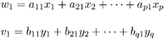
such that the two canonical variables, w ₁ and v ₁ , have the largest possible correlation. This maximized correlation between the two canonical variables is the first canonical correlation. The coefficients of the linear combinations are canonical coefficients or canonical weights. It is customary to normalize the canonical coefficients so that each canonical variable has a variance of 1.

PROC CANCORR continues by finding a second set of canonical variables, uncorrelated with the first pair, that produces the second highest correlation coefficient. That is, the second pair of canonical variables is:

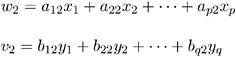
such that w ₂ is uncorrelated with w ₁ and v ₁ , v ₂ is uncorrelated with w ₁ and v ₁ , and w ₂ and v ₂ have the largest possible correlation subject to these constraints. The process of constructing canonical variables continues until the number of pairs of canonical variables is min( p, q ), the number of variables in the smaller group.

Each canonical variable is uncorrelated with all the other canonical variables of either set except for the one corresponding canonical variable in the opposite set. The canonical coefficients are not generally orthogonal, however, so the canonical variables do not represent jointly perpendicular directions through the space of the original variables.

The first canonical correlation is at least as large as the multiple correlation between any variable and the opposite set of variables. It is possible for the first canonical correlation to be very large while all the multiple correlations for predicting one of the original variables from the opposite set of canonical variables are small. Canonical redundancy analysis (Stewart and Love 1968; Cooley and Lohnes 1971; van den Wollenberg 1977), examines how well the original variables can be predicted from the canonical variables.

PROC CANCORR can also perform partial canonical correlation, which is a multivariate generalization of ordinary partial correlation (Cooley and Lohnes 1971; Timm 1975). Most commonly-used parametric statistical methods , ranging from t tests to multivariate analysis of covariance, are special cases of partial canonical correlation.