Syntax | SAS/STAT 9.1 Users Guide, Volumes 1-7

The following statements are available in PROC ANOVA.

PROC ANOVA < options > ;
- CLASS variables < / option > ;
- MODEL dependents=effects < / options > ;
- ABSORB variables ;
- BY variables ;
- FREQ variable ;
- MANOVA < test-options >< / detail-options > ;
- MEANS effects < / options > ;
- REPEATED factor-specification < / options > ;
- TEST < H= effects > E= effect ;

The PROC ANOVA, CLASS, and MODEL statements are required, and they must precede the first RUN statement. The CLASS statement must precede the MODEL statement. If you use the ABSORB, FREQ, or BY statement, it must precede the first RUN statement. The MANOVA, MEANS, REPEATED, and TEST statements must follow the MODEL statement, and they can be specified in any order. These four statements can also appear after the first RUN statement.

The following table summarizes the function of each statement (other than the PROC statement) in the ANOVA procedure:

Table 17.1: Statements in the ANOVA Procedure
Statement	Description
ABSORB	absorbs classification effects in a model
BY	specifies variables to define subgroups for the analysis
CLASS	declares classification variables
FREQ	specifies a frequency variable
MANOVA	performs a multivariate analysis of variance
MEANS	computes and compares means
MODEL	defines the model to be fit
REPEATED	performs multivariate and univariate repeated measures analysis of variance
TEST	constructs tests using the sums of squares for effects and the error term you specify

PROC ANOVA Statement

PROC ANOVA < options > ;

The PROC ANOVA statement starts the ANOVA procedure.

You can specify the following options in the PROC ANOVA statement:

DATA= SAS-data-set

names the SAS data set used by the ANOVA procedure. By default, PROC ANOVA uses the most recently created SAS data set.

MANOVA

requests the multivariate mode of eliminating observations with missing values. If any of the dependent variables have missing values, the procedure eliminates that observation from the analysis. The MANOVA option is useful if you use PROC ANOVA in interactive mode and plan to perform a multivariate analysis.

MULTIPASS

requests that PROC ANOVA reread the input data set, when necessary, instead of writing the values of dependent variables to a utility file. This option decreases disk space usage at the expense of increased execution times and is useful only in rare situations where disk space is at an absolute premium.

NAMELEN= n

specifies the length of effect names to be n characters long, where n is a value between 20 and 200 characters. The default length is 20 characters.

NOPRINT

suppresses the normal display of results. The NOPRINT option is useful when you want to create only the output data set with the procedure. Note that this option temporarily disables the Output Delivery System (ODS); see Chapter 14, 'Using the Output Delivery System,' for more information.

ORDER=DATA FORMATTED FREQ INTERNAL

specifies the sorting order for the levels of the classification variables (specified in the CLASS statement). This ordering determines which parameters in the model correspond to each level in the data. Note that the ORDER= option applies to the levels for all classification variables. The exception is the default ORDER=FORMATTED for numeric variables for which you have supplied no explicit format. In this case, the levels are ordered by their internal value. Note that this represents a change from previous releases for how class levels are ordered. In releases previous to Version 8, numeric class levels with no explicit format were ordered by their BEST12. formatted values, and in order to revert to the previous ordering you can specify this format explicitly for the affected classification variables. The change was implemented because the former default behavior for ORDER=FORMATTED often resulted in levels not being ordered numerically and usually required the user to intervene with an explicit format or ORDER=INTERNAL to get the more natural ordering.

The following table shows how PROC ANOVA interprets values of the ORDER= option.

Value of ORDER=	Levels Sorted By
DATA	order of appearance in the input data set
FORMATTED	external formatted value, except for numeric variables with no explicit format, which are sorted by their unformatted (internal) value
FREQ	descending frequency count; levels with the most observations come first in the order
INTERNAL	unformatted value

OUTSTAT= SAS-data-set

names an output data set that contains sums of squares, degrees of freedom, F statistics, and probability levels for each effect in the model. If you use the CANONICAL option in the MANOVA statement and do not use an M= specificationinthe MANOVA statement, the data set also contains results of the canonical analysis. See the 'Output Data Set' section on page 455 for more information.

ABSORB Statement

ABSORB variables ;

Absorption is a computational technique that provides a large reduction in time and memory requirements for certain types of models. The variables are one or more variables in the input data set.

For a main effect variable that does not participate in interactions, you can absorb the effect by naming it in an ABSORB statement. This means that the effect can be adjusted out before the construction and solution of the rest of the model. This is particularly useful when the effect has a large number of levels.

Several variables can be specified, in which case each one is assumed to be nested in the preceding variable in the ABSORB statement.

Note: When you use the ABSORB statement, the data set (or each BY group , if a BY statement appears) must be sorted by the variables in the ABSORB statement. Including an absorbed variable in the CLASS list or in the MODEL statement may produce erroneous sums of squares. If the ABSORB statement is used, it must appear before the first RUN statement or it is ignored.

When you use an ABSORB statement and also use the INT option in the MODEL statement, the procedure ignores the option but produces the uncorrected total sum of squares (SS) instead of the corrected total SS.

See the 'Absorption' section on page 1799 in Chapter 32, 'The GLM Procedure,' for more information.

BY Statement

BY variables ;

You can specify a BY statement with PROC ANOVA to obtain separate analyses on observations in groups defined by the BY variables. When a BY statement appears, the procedure expects the input data set to be sorted in order of the BY variables. The variables are one or more variables in the input data set.

If your input data set is not sorted in ascending order, use one of the following alternatives:

Sort the data using the SORT procedure with a similar BY statement.
Specify the BY statement option NOTSORTED or DESCENDING in the BY statement for the ANOVA procedure. The NOTSORTED option does not mean that the data are unsorted but rather that the data are arranged in groups (according to values of the BY variables) and that these groups are not necessarily in alphabetical or increasing numeric order.
Create an index on the BY variables using the DATASETS procedure (in base SAS software).

Since sorting the data changes the order in which PROC ANOVA reads observations, the sorting order for the levels of the classification variables may be affected if you have also specified the ORDER=DATA option in the PROC ANOVA statement.

If the BY statement is used, it must appear before the first RUN statement or it is ignored. When you use a BY statement, the interactive features of PROC ANOVA are disabled.

When both a BY and an ABSORB statement are used, observations must be sorted first by the variables in the BY statement, and then by the variables in the ABSORB statement.

For more information on the BY statement, refer to the discussion in SAS Language Reference: Concepts . For more information on the DATASETS procedure, refer to the discussion in the SAS Procedures Guide .

CLASS Statement

CLASS variables < / option > ;

The CLASS statement names the classification variables to be used in the model. Typical class variables are TREATMENT, SEX, RACE, GROUP, and REPLICATION. The CLASS statement is required, and it must appear before the MODEL statement.

By default, class levels are determined from the entire formatted values of the CLASS variables. Note that this represents a slight change from previous releases in the way in which class levels are determined. In releases prior to Version 9, class levels were determined using no more than the first 16 characters of the formatted values. If you wish to revert to this previous behavior you can use the TRUNCATE option on the CLASS statement. In any case, you can use formats to group values into levels. Refer to the discussion of the FORMAT procedure in the SAS Procedures Guide and the discussions for the FORMAT statement and SAS formats in SAS Language Reference: Concepts .

You can specify the following option in the CLASS statement after a slash(/):

TRUNCATE

specifies that class levels should be determined using only up to the first 16 characters of the formatted values of CLASS variables. When formatted values are longer than 16 characters, you can use this option in order to revert to the levels as determined in releases previous to Version 9.

FREQ Statement

FREQ variable ;

The FREQ statement names a variable that provides frequencies for each observation in the DATA= data set. Specifically, if n is the value of the FREQ variable for a given observation, then that observation is used n times.

The analysis produced using a FREQ statement reflects the expanded number of observations. For example, means and total degrees of freedom reflect the expanded number of observations. You can produce the same analysis (without the FREQ statement) by first creating a new data set that contains the expanded number of observations. For example, if the value of the FREQ variable is 5 for the first observation, the first 5 observations in the new data set would be identical. Each observation in the old data set would be replicated n _i times in the new data set, where n _i is the value of the FREQ variable for that observation.

If the value of the FREQ variable is missing or is less than 1, the observation is not used in the analysis. If the value is not an integer, only the integer portion is used.

If the FREQ statement is used, it must appear before the first RUN statement or it is ignored.

MANOVA Statement

MANOVA < test-options >< / detail-options > ;

If the MODEL statement includes more than one dependent variable, you can perform multivariate analysis of variance with the MANOVA statement. The test-options define which effects to test, while the detail-options specify how to execute the tests and what results to display.

When a MANOVA statement appears before the first RUN statement, PROC ANOVA enters a multivariate mode with respect to the handling of missing values; in addition to observations with missing independent variables, observations with any missing dependent variables are excluded from the analysis. If you want to use this mode of handling missing values but do not need any multivariate analyses, specify the MANOVA option in the PROC ANOVA statement.

Test Options

You can specify the following options in the MANOVA statement as test-options in order to define which multivariate tests to perform.

H= effects INTERCEPT _ ALL_

specifies effects in the preceding model to use as hypothesis matrices. For each SSCP matrix H associated with an effect, the H= specification computes an analysis based on the characteristic roots of E ^{ˆ’ 1} H , where E is the matrix associated with the error effect. The characteristic roots and vectors are displayed, along with the Hotelling-Lawley trace, Pillai's trace, Wilks' criterion, and Roy's maximum root criterion with approximate F statistics. By default, these statistics are tested with approximations based on the F distribution. To test them with exact (but computationally intensive ) calculations, use the MSTAT=EXACT option.

Use the keyword INTERCEPT to produce tests for the intercept. To produce tests for all effects listed in the MODEL statement, use the keyword _ALL_ in place of a list of effects. For background and further details, see the 'Multivariate Analysis of Variance' section on page 1823 in Chapter 32, 'The GLM Procedure.'

E= effect

specifies the error effect. If you omit the E= specification, the ANOVA procedure uses the error SSCP ( residual ) matrix from the analysis.

M= equation, ... ,equation ( row-of-matrix, ... ,row-of-matrix )

specifies a transformation matrix for the dependent variables listed in the MODEL statement. The equations in the M= specification are of the form

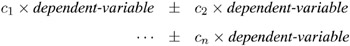
where the c _i values are coefficients for the various dependent-variables . If the value of a given c _i is 1, it may be omitted; in other words 1 — Y is the same as Y . Equations should involve two or more dependent variables. For sample syntax, see the 'Examples' section on page 439.

Alternatively, you can input the transformation matrix directly by entering the elements of the matrix with commas separating the rows, and parentheses surrounding the matrix. When this alternate form of input is used, the number of elements in each row must equal the number of dependent variables. Although these combinations actually represent the columns of the M matrix, they are displayed by rows.

When you include an M= specification, the analysis requested in the MANOVA statement is carried out for the variables defined by the equations in the specification, not the original dependent variables. If you omit the M= option, the analysis is performed for the original dependent variables in the MODEL statement.

If an M= specification is included without either the MNAMES= or the PREFIX= option, the variables are labeled MVAR1, MVAR2, and so forth by default. For further information, see the section 'Multivariate Analysis of Variance' on page 1823 in Chapter 32, 'The GLM Procedure.'

MNAMES= names

provides names for the variables defined by the equations in the M= specification. Names in the list correspond to the M= equations or the rows of the M matrix (as it is entered).

PREFIX= name

is an alternative means of identifying the transformed variables definedbytheM= specification. For example, if you specify PREFIX=DIFF, the transformed variables are labeled DIFF1, DIFF2, and so forth.

Detail Options

You can specify the following options in the MANOVA statement after a slash as detail-options :

CANONICAL

produces a canonical analysis of the H and E matrices (transformed by the M matrix, if specified) instead of the default display of characteristic roots and vectors.

MSTAT=FAPPROX

MSTAT=EXACT

specifies the method of evaluating the multivariate test statistics. The default is MSTAT=FAPPROX, which specifies that the multivariate tests are evaluated using the usual approximations based on the F distribution, as discussed in the 'Multivariate Tests' section in Chapter 2, 'Introduction to Regression Procedures.' Alternatively, you can specify MSTAT=EXACT to compute exact p -values for three of the four tests (Wilks' Lambda, the Hotelling-Lawley Trace, and Roy's Greatest Root) and an improved F- approximation for the fourth (Pillai's Trace). While MSTAT=EXACT provides better control of the significance probability for the tests, especially for Roy's Greatest Root, computations for the exact p -values can be appreciably more demanding, and are in fact infeasible for large problems (many dependent variables). Thus, although MSTAT=EXACT is more accurate for most data, it is not the default method. For more information on the results of MSTAT=EXACT, see the 'Multivariate Analysis of Variance' section on page 1823 in Chapter 32, 'The GLM Procedure.'

ORTH

requests that the transformation matrix in the M= specification of the MANOVA statement be orthonormalized by rows before the analysis.

PRINTE

displays the error SSCP matrix E . If the E matrix is the error SSCP (residual) matrix from the analysis, the partial correlations of the dependent variables given the independent variables are also produced.

For example, the statement
```
  manova / printe;  
```
displays the error SSCP matrix and the partial correlation matrix computed from the error SSCP matrix.

PRINTH

displays the hypothesis SSCP matrix H associated with each effect specified by the H= specification.

SUMMARY

produces analysis-of-variance tables for each dependent variable. When no M matrix is specified, a table is produced for each original dependent variable from the MODEL statement; with an M matrix other than the identity, a table is produced for each transformed variable defined by the M matrix.

Examples

The following statements give several examples of using a MANOVA statement.

  proc anova;   class A B;   model Y1-Y5=A B(A);   manova h=A e=B(A) / printh printe;   manova h=B(A) / printe;   manova h=A e=B(A) m=Y1-Y2,Y2-Y3,Y3-Y4,Y4-Y5   prefix=diff;   manova h=A e=B(A) m=(1   1  0  0  0,   0  1   1  0  0,   0  0  1   1  0,   0  0  0  1   1) prefix=diff;   run;

The first MANOVA statement specifies A as the hypothesis effect and B ( A )asthe error effect. As a result of the PRINTH option, the procedure displays the hypothesis SSCP matrix associated with the A effect; and, as a result of the PRINTE option, the procedure displays the error SSCP matrix associated with the B ( A ) effect.

The second MANOVA statement specifies B ( A ) as the hypothesis effect. Since no error effect is specified, PROC ANOVA uses the error SSCP matrix from the analysis as the E matrix. The PRINTE option displays this E matrix. Since the E matrix is the error SSCP matrix from the analysis, the partial correlation matrix computed from this matrix is also produced.

The third MANOVA statement requests the same analysis as the first MANOVA statement, but the analysis is carried out for variables transformed to be successive differences between the original dependent variables. The PREFIX=DIFF specification labels the transformed variables as DIFF1, DIFF2, DIFF3, and DIFF4.

Finally, the fourth MANOVA statement has the identical effect as the third, but it uses an alternative form of the M= specification. Instead of specifying a set of equations, the fourth MANOVA statement specifies rows of a matrix of coefficients for the five dependent variables.

As a second example of the use of the M= specification, consider the following:

  proc anova;   class group;   model dose1-dose4=group / nouni;   manova h = group   m =   3*dose1   dose2 +   dose3 + 3*dose4,   dose1   dose2   dose3 +   dose4,   -dose1  + 3*dose2   3*dose3 +   dose4   mnames = Linear Quadratic Cubic   / printe;   run;

The M= specification gives a transformation of the dependent variables dose1 through dose4 into orthogonal polynomial components, and the MNAMES= option labels the transformed variables as LINEAR, QUADRATIC, and CUBIC, respectively. Since the PRINTE option is specified and the default residual matrix is used as an error term, the partial correlation matrix of the orthogonal polynomial components is also produced.

For further information, see the 'Multivariate Analysis of Variance' section on page 1823 in Chapter 32, 'The GLM Procedure.'

MEANS Statement

MEANS effects < / options > ;

PROC ANOVA can compute means of the dependent variables for any effect that appears on the right-hand side in the MODEL statement.

You can use any number of MEANS statements, provided that they appear after the MODEL statement. For example, suppose A and B each have two levels. Then, if you use the following statements

  proc anova;   class A B;   model Y=A B A*B;   meansA B / tukey;   means A*B;   run;

means, standard deviations, and Tukey's multiple comparison tests are produced for each level of the main effects A and B , and just the means and standard deviations for each of the four combinations of levels for A * B . Since multiple comparisons options apply only to main effects, the single MEANS statement

  means A B A*B / tukey;

produces the same results.

Options are provided to perform multiple comparison tests for only main effects in the model. PROC ANOVA does not perform multiple comparison tests for interaction terms in the model; for multiple comparisons of interaction terms, see the LSMEANS statement in Chapter 32, 'The GLM Procedure.'

The following table summarizes categories of options available in the MEANS statement.

Table 17.2: Options Available in the MEANS Statement
Task	Available options
Perform multiple comparison tests	BON DUNCAN DUNNETT DUNNETTL DUNNETTU GABRIEL GT2 LSD REGWQ SCHEFFE SIDAK SMM
Perform multiple comparison tests	SNK T TUKEY WALLER
Specify additional details for multiple comparison tests	ALPHA= CLDIFF CLM E= KRATIO= LINES NOSORT
Test for homogeneity of variances	HOVTEST
Compensate for heterogeneous variances	WELCH

Descriptions of these options follow. For a further discussion of these options, see the section 'Multiple Comparisons' on page 1806 in Chapter 32, 'The GLM Procedure.'

ALPHA= p

specifies the level of significance for comparisons among the means. By default, ALPHA=0.05. You can specify any value greater than 0 and less than 1.

BON

performs Bonferroni t tests of differences between means for all main effect means in the MEANS statement. See the CLDIFF and LINES options, which follow, for a discussion of how the procedure displays results.

CLDIFF

presents results of the BON, GABRIEL, SCHEFFE, SIDAK, SMM, GT2, T, LSD, and TUKEY options as confidence intervals for all pairwise differences between means, and the results of the DUNNETT, DUNNETTU, and DUNNETTL options as confidence intervals for differences with the control. The CLDIFF option is the default for unequal cell sizes unless the DUNCAN, REGWQ, SNK, or WALLER option is specified.

CLM

presents results of the BON, GABRIEL, SCHEFFE, SIDAK, SMM, T, and LSD options as intervals for the mean of each level of the variables specified in the MEANS statement. For all options except GABRIEL, the intervals are confidence intervals for the true means. For the GABRIEL option, they are comparison intervals for comparing means pairwise: in this case, if the intervals corresponding to two means overlap, the difference between them is insignificant according to Gabriel's method.

DUNCAN

performs Duncan's multiple range test on all main effect means given in the MEANS statement. See the LINES option for a discussion of how the procedure displays results.

DUNNETT < ( formatted-control-values ) >

performs Dunnett's two-tailed t test, testing if any treatments are significantly different from a single control for all main effects means in the MEANS statement. To specify which level of the effect is the control, enclose the formatted value in quotes in parentheses after the keyword. If more than one effect is specified in the MEANS statement, you can use a list of control values within the parentheses. By default, the first level of the effect is used as the control. For example,
```
  means a / dunnett('CONTROL');  
```
where CONTROL is the formatted control value of A. As another example,
```
  means a b c / dunnett('CNTLA' 'CNTLB' 'CNTLC');  
```
where CNTLA, CNTLB, and CNTLC are the formatted control values for A, B, and C, respectively.

DUNNETTL < ( formatted-control-value ) >

performs Dunnett's one-tailed t test, testing if any treatment is significantly less than the control. Control level information is specified as described previously for the DUNNETT option.

DUNNETTU < ( formatted-control-value ) >

performs Dunnett's one-tailed t test, testing if any treatment is significantly greater than the control. Control level information is specified as described previously for the DUNNETT option.

E= effect

specifies the error mean square used in the multiple comparisons. By default, PROC ANOVA uses the residual Mean Square (MS). The effect specified with the E= option must be a term in the model; otherwise , the procedure uses the residual MS.

GABRIEL

performs Gabriel's multiple-comparison procedure on all main effect means in the MEANS statement. See the CLDIFF and LINES options for discussions of how the procedure displays results.

GT2

see the SMM option.

HOVTEST

HOVTEST=BARTLETT

HOVTEST=BF

HOVTEST=LEVENE < (TYPE=ABS SQUARE) >

HOVTEST=OBRIEN < (W= number ) >

requests a homogeneity of variance test for the groups defined by the MEANS effect. You can optionally specify a particular test; if you do not specify a test, Levene's test (Levene 1960) with TYPE=SQUARE is computed. Note that this option is ignored unless your MODEL statement specifies a simple one-way model.

The HOVTEST=BARTLETT option specifies Bartlett's test (Bartlett 1937), a modification of the normal-theory likelihood ratio test.

The HOVTEST=BF option specifies Brown and Forsythe's variation of Levene's test (Brown and Forsythe 1974).

The HOVTEST=LEVENE option specifies Levene's test (Levene 1960), which is widely considered to be the standard homogeneity of variance test. You can use the TYPE= option in parentheses to specify whether to use the absolute residuals (TYPE=ABS) or the squared residuals (TYPE=SQUARE) in Levene's test. The default is TYPE=SQUARE.

The HOVTEST=OBRIEN option specifies O'Brien's test (O'Brien 1979), which is basically a modification of HOVTEST=LEVENE(TYPE=SQUARE). You can use the W= option in parentheses to tune the variable to match the suspected kurtosis of the underlying distribution. By default, W=0.5, as suggested by O'Brien (1979, 1981).

See the section 'Homogeneity of Variance in One-Way Models' on page 1818 in Chapter 32, 'The GLM Procedure,' for more details on these methods . Example 32.10 on page 1892 in the same chapter illustrates the use of the HOVTEST and WELCH options in the MEANS statement in testing for equal group variances.

KRATIO= value

specifies the Type 1/Type 2 error seriousness ratio for the Waller-Duncan test. Reasonable values for KRATIO are 50, 100, and 500, which roughly correspond for the two-level case to ALPHA levels of 0.1, 0.05, and 0.01. By default, the procedure uses the default value of 100.

LINES

presents results of the BON, DUNCAN, GABRIEL, REGWQ, SCHEFFE, SIDAK, SMM, GT2, SNK, T, LSD, TUKEY, and WALLER options by listing the means in descending order and indicating nonsignificant subsets by line segments beside the corresponding means. The LINES option is appropriate for equal cell sizes, for which it is the default. The LINES option is also the default if the DUNCAN, REGWQ, SNK, or WALLER option is specified, or if there are only two cells of unequal size . If the cell sizes are unequal, the harmonic mean of the cell sizes is used, which may lead to somewhat liberal tests if the cell sizes are highly disparate. The LINES option cannot be used in combination with the DUNNETT, DUNNETTL, or DUNNETTU option. In addition, the procedure has a restriction that no more than 24 overlapping groups of means can exist. If a mean belongs to more than 24 groups, the procedure issues an error message. You can either reduce the number of levels of the variable or use a multiple comparison test that allows the CLDIFF option rather than the LINES option.

LSD

see the T option.

NOSORT

prevents the means from being sorted into descending order when the CLDIFF or CLM option is specified.

REGWQ

performs the Ryan-Einot-Gabriel-Welsch multiple range test on all main effect means in the MEANS statement. See the LINES option for a discussion of how the procedure displays results.

SCHEFFE

performs Scheff 's multiple-comparison procedure on all main effect means in the MEANS statement. See the CLDIFF and LINES options for discussions of how the procedure displays results.

SIDAK

performs pairwise t tests on differences between means with levels adjusted according to Sidak's inequality for all main effect means in the MEANS statement. See the CLDIFF and LINES options for discussions of how the procedure displays results.

SMM

GT2

performs pairwise comparisons based on the studentized maximum modulus and Sidak's uncorrelated- t inequality, yielding Hochberg's GT2 method when sample sizes are unequal, for all main effect means in the MEANS statement. See the CLDIFF and LINES options for discussions of how the procedure displays results.

SNK

performs the Student-Newman-Keuls multiple range test on all main effect means in the MEANS statement. See the LINES option for a discussion of how the procedure displays results.

LSD

performs pairwise t tests, equivalent to Fisher's least-significant-difference test in the case of equal cell sizes, for all main effect means in the MEANS statement. See the CLDIFF and LINES options for discussions of how the procedure displays results.

TUKEY

performs Tukey's studentized range test (HSD) on all main effect means in the MEANS statement. (When the group sizes are different, this is the Tukey-Kramer test.) See the CLDIFF and LINES options for discussions of how the procedure displays results.

WALLER

performs the Waller-Duncan k -ratio t test on all main effect means in the MEANS statement. See the KRATIO= option for information on controlling details of the test, and see the LINES option for a discussion of how the procedure displays results.

WELCH

requests Welch's (1951) variance-weighted one-way ANOVA. This alternative to the usual analysis of variance for a one-way model is robust to the assumption of equal within-group variances. This option is ignored unless your MODEL statement specifies a simple one-way model.

Note that using the WELCH option merely produces one additional table consisting of Welch's ANOVA. It does not affect all of the other tests displayed by the ANOVA procedure, which still require the assumption of equal variance for exact validity.

See the 'Homogeneity of Variance in One-Way Models' section on page 1818 in Chapter 32, 'The GLM Procedure,' for more details on Welch's ANOVA. Example 32.10 on page 1892 in the same chapter illustrates the use of the HOVTEST and WELCH options in the MEANS statement in testing for equal group variances.

MODEL Statement

MODEL dependents=effects < / options > ;

The MODEL statement names the dependent variables and independent effects. The syntax of effects is described in the section 'Specification of Effects' on page 451. For any model effect involving classification variables (interactions as well as main effects), the number of levels can not exceed 32,767. If no independent effects are specified, only an intercept term is fit. This tests the hypothesis that the mean of the dependent variable is zero. All variables in effects that you specify in the MODEL statement must appear in the CLASS statement because PROC ANOVA does not allow for continuous effects.

You can specify the following options in the MODEL statement; they must be separated from the list of independent effects by a slash.

INTERCEPT

INT

displays the hypothesis tests associated with the intercept as an effect in the model. By default, the procedure includes the intercept in the model but does not display associated tests of hypotheses. Except for producing the uncorrected total SS instead of the corrected total SS, the INT option is ignored when you use an ABSORB statement.

NOUNI

suppresses the display of univariate statistics. You typically use the NOUNI option with a multivariate or repeated measures analysis of variance when you do not need the standard univariate output. The NOUNI option in a MODEL statement does not affect the univariate output produced by the REPEATED statement.

REPEATED Statement

REPEATED factor-specification < / options > ;

When values of the dependent variables in the MODEL statement represent repeated measurements on the same experimental unit, the REPEATED statement enables you to test hypotheses about the measurement factors (often called within-subject factors ), as well as the interactions of within-subject factors with independent variables in the MODEL statement (often called between-subject factors ). The REPEATED statement provides multivariate and univariate tests as well as hypothesis tests for a variety of single-degree-of-freedom contrasts. There is no limit to the number of within-subject factors that can be specified. For more details, see the 'Repeated Measures Analysis of Variance' section on page 1825 in Chapter 32, 'The GLM Procedure.'

The REPEATED statement is typically used for handling repeated measures designs with one repeated response variable. Usually, the variables on the left-hand side of the equation in the MODEL statement represent one repeated response variable. This does not mean that only one factor can be listed in the REPEATED statement. For example, one repeated response variable (hemoglobin count) might be measured 12 times (implying variables Y1 to Y12 on the left-hand side of the equal sign in the MODEL statement), with the associated within-subject factors treatment and time ( implying two factors listed in the REPEATED statement). See the 'Examples' section on page 449 for an example of how PROC ANOVA handles this case. Designs with two or more repeated response variables can, however, be handled with the IDENTITY transformation;see Example 32.9 on page 1886 in Chapter 32, 'The GLM Procedure,' for an example of analyzing a doubly-multivariate repeated measures design.

When a REPEATED statement appears, the ANOVA procedure enters a multivariate mode of handling missing values. If any values for variables corresponding to each combination of the within-subject factors are missing, the observation is excluded from the analysis.

The simplest form of the REPEATED statement requires only a factor-name . With two repeated factors, you must specify the factor-name and number of levels ( levels ) for each factor. Optionally, you can specify the actual values for the levels ( level-values ), a transformation that defines single-degree-of freedom contrasts, and options for additional analyses and output. When more than one within-subject factor is specified, factor-names (and associated level and transformation information) must be separated by a comma in the REPEATED statement. These terms are described in the following section, 'Syntax Details.'

Syntax Details

You can specify the following terms in the REPEATED statement.

factor-specification

The factor-specification for the REPEATED statement can include any number of individual factor specifications, separated by commas, of the following form:
- factor-name levels < ( level-values ) >< transformation >

where

factor-name

names a factor to be associated with the dependent variables. The name should not be the same as any variable name that already exists in the data set being analyzed and should conform to the usual conventions of SAS variable names.

levels

specifies the number of levels associated with the factor being defined. When there is only one within-subject factor, the number of levels is equal to the number of dependent variables. In this case, levels is optional. When more than one within-subject factor is defined, however, levels is required, and the product of the number of levels of all the factors must equal the number of dependent variables in the MODEL statement.

(level-values)

specifies values that correspond to levels of a repeated-measures factor. These values are used to label output; they are also used as spacings for constructing orthogonal polynomial contrasts if you specify a POLYNOMIAL transformation. The number of level values specified must correspond to the number of levels for that factor in the REPEATED statement. Enclose the level-values in parentheses.

The following transformation keywords define single-degree-of-freedom contrasts for factors specified in the REPEATED statement. Since the number of contrasts generated is always one less than the number of levels of the factor, you have some control over which contrast is omitted from the analysis by which transformation you select. The only exception is the IDENTITY transformation; this transformation is not composed of contrasts, and it has the same degrees of freedom as the factor has levels. By default, the procedure uses the CONTRAST transformation.

CONTRAST < ( ordinal-reference-level ) >	generates contrasts between levels of the factor and a reference level. By default, the procedure uses the last level; you can optionally specify a reference level in parentheses after the keyword CONTRAST. The reference level corresponds to the ordinal value of the level rather than the level value specified. For example, to generate contrasts between the first level of a factor and the other levels, use contrast(1)
HELMERT	generates contrasts between each level of the factor and the mean of subsequent levels.
IDENTITY	generates an identity transformation corresponding to the associated factor. This transformation is not composed of contrasts; it has n degrees of freedom for an n -level factor, instead of n ˆ’ 1. This can be used for doubly-multivariate repeated measures.
MEAN < ( ordinal-reference-level ) >	generates contrasts between levels of the factor and the mean of all other levels of the factor. Specifying a reference level eliminates the contrast between that level and the mean. Without a reference level, the contrast involving the last level is omitted. See the CONTRAST transformation for an example.
POLYNOMIAL	generates orthogonal polynomial contrasts. Level values, if provided, are used as spacings in the construction of the polynomials ; otherwise, equal spacing is assumed.
PROFILE	generates contrasts between adjacent levels of the factor.

For examples of the transformation matrices generated by these contrast transformations, see the section 'Repeated Measures Analysis of Variance' on page 1825 in Chapter 32, 'The GLM Procedure.'

You can specify the following options in the REPEATED statement after a slash:

CANONICAL

performs a canonical analysis of the H and E matrices corresponding to the transformed variables specified in the REPEATED statement.

MSTAT=FAPPROX

MSTAT=EXACT

specifies the method of evaluating the multivariate test statistics. The default is MSTAT=FAPPROX, which specifies that the multivariate tests are evaluated using the usual approximations based on the F distribution, as discussed in the 'Multivariate Tests' section in Chapter 2, 'Introduction to Regression Procedures.' Alternatively, you can specify MSTAT=EXACT to compute exact p -values for three of the four tests (Wilks' Lambda, the Hotelling-Lawley Trace, and Roy's Greatest Root) and an improved F-approximation for the fourth (Pillai's Trace). While MSTAT=EXACT provides better control of the significance probability for the tests, especially for Roy's Greatest Root, computations for the exact p -values can be appreciably more demanding, and are in fact infeasible for large problems (many dependent variables). Thus, although MSTAT=EXACT is more accurate for most data, it is not the default method. For more information on the results of MSTAT=EXACT, see the 'Multivariate Analysis of Variance' section on page 1823 in Chapter 32, 'The GLM Procedure.' .

NOM

displays only the results of the univariate analyses.

NOU

displays only the results of the multivariate analyses.

PRINTE

displays the E matrix for each combination of within-subject factors, as well as partial correlation matrices for both the original dependent variables and the variables defined by the transformations specified in the REPEATED statement. In addition, the PRINTE option provides sphericity tests for each set of transformed variables. If the requested transformations are not orthogonal, the PRINTE option also provides a sphericity test for a set of orthogonal contrasts.

PRINTH

displays the H (SSCP) matrix associated with each multivariate test.

PRINTM

displays the transformation matrices that define the contrasts in the analysis. PROC ANOVA always displays the M matrix so that the transformed variables are defined by the rows, not the columns, of the displayed M matrix. In other words, PROC ANOVA actually displays M ² .

PRINTRV

produces the characteristic roots and vectors for each multivariate test.

SUMMARY

produces analysis-of-variance tables for each contrast defined by the within-subjects factors. Along with tests for the effects of the independent variables specified in the MODEL statement, a term labeled MEAN tests the hypothesis that the overall mean of the contrast is zero.

Examples

When specifying more than one factor, list the dependent variables in the MODEL statement so that the within-subject factors defined in the REPEATED statement are nested; that is, the first factor defined in the REPEATED statement should be the one with values that change least frequently. For example, assume that three treatments are administered at each of four times, for a total of twelve dependent variables on each experimental unit. If the variables are listed in the MODEL statement as Y1 through Y12 , then the following REPEATED statement

  repeated trt 3, time 4;

implies the following structure:

	Dependent Variables
	Y1	Y2	Y3	Y4	Y5	Y6	Y7	Y8	Y9	Y10	Y11	Y12
Value of trt	1	1	1	1	2	2	2	2	3	3	3	3
Value of time	1	2	3	4	1	2	3	4	1	2	3	4

The REPEATED statement always produces a table like the preceding one. For more information on repeated measures analysis and on using the REPEATED statement, see the section 'Repeated Measures Analysis of Variance' on page 1825 in Chapter 32, 'The GLM Procedure.'

TEST Statement

TEST < H= effects > E= effect ;

Although an F value is computed for all SS in the analysis using the residual MS as an error term, you can request additional F tests using other effects as error terms. You need a TEST statement when a nonstandard error structure (as in a split plot) exists.

Caution: The ANOVA procedure does not check any of the assumptions underlying the F statistic. When you specify a TEST statement, you assume sole responsibility for the validity of the F statistic produced. To help validate a test, you may want to use the GLM procedure with the RANDOM statement and inspect the expected mean squares. In the GLM procedure, you can also use the TEST option in the RANDOM statement.

You can use as many TEST statements as you want, provided that they appear after the MODEL statement.

You can specify the following terms in the TEST statement.

H= effects	specifies which effects in the preceding model are to be used as hypothesis (numerator) effects.
E= effect	specifies one, and only one, effect to use as the error (denominator) term. The E= specification is required.

The following example uses two TEST statements and is appropriate for analyzing a split-plot design.

  proc anova;   class a b c;   model y=ab(a)c;   test h=a e=b(a);   test h=c a*c e=b*c(a);   run;