Section 2.1. Common Kernel Datatypes

2.1. Common Kernel Datatypes

The Linux kernel has many objects and structures of which to keep track. Examples include memory pages, processes, and interrupts. A timely way to reference one of these objects among many is a major concern if the operating system is run efficiently. Linux uses linked lists and binary search trees (along with a set of helper routines) to first group these objects into a single container and, second, to find a single element in an efficient manner.

2.1.1. Linked Lists

Linked lists are common datatypes in computer science and are used throughout the Linux kernel. Linked lists are often implemented as circular doubly linked lists within the Linux kernel. (See Figure 2.1.) Thus, given any node in a list, we can go to the next or previous node. All the code for linked lists can be viewed in include/linux/list.h. This section deals with the major features of linked lists.

Figure 2.1. Linked List After the INIT_LIST_HEAD Macro Is Called

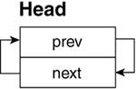
A linked list is initialized by using the LIST_HEAD and INIT_ LIST_HEAD macros:

 ----------------------------------------------------------------------------- include/linux/list.h 27 28 struct list_head { 29   struct list_head *next, *prev; 30 }; 31  32 #define LIST_HEAD_INIT(name) { &(name), &(name) } 33  34 #define LIST_HEAD(name) \ 35   struct list_head name = LIST_HEAD_INIT(name) 36  37 #define INIT_LIST_HEAD(ptr) do { \ 38   (ptr)->next = (ptr); (ptr)->prev = (ptr); \ 39 } while (0) ----------------------------------------------------------------------------- 

Line 34

The LIST_HEAD macro creates the linked list head specified by name.

Line 37

The INIT_LIST_HEAD macro initializes the previous and next pointers within the structure to reference the head itself. After both of these calls, name contains an empty doubly linked list.^[2]

^[2] An empty list is defined as one whose head->next field points to the list's head element.

Simple stacks and queues can be implemented by the list_add() or list_add_tail() functions, respectively. A good example of this being used is in the work queue code:

 ----------------------------------------------------------------------------- kernel/workqueue.c 330 list_add(&wq->list, &workqueues); ----------------------------------------------------------------------------- 

The kernel adds wq->list to the system-wide list of work queues, workqueues. workqueues is thus a stack of queues.

Similarly, the following code adds work->entry to the end of the list cwq->worklist. cwq->worklist is thus being treated as a queue:

 ----------------------------------------------------------------------------- kernel/workqueue.c 84 list_add_tail(&work->entry, &cwq->worklist); ----------------------------------------------------------------------------- 

When deleting an element from a list, list_del() is used. list_del() takes the list entry as a parameter and deletes the element simply by modifying the entry's next and previous nodes to point to each other. For example, when a work queue is destroyed, the following code removes the work queue from the system-wide list of work queues:

 ----------------------------------------------------------------------------- kernel/workqueue.c 382 list_del(&wq->list); ----------------------------------------------------------------------------- 

One extremely useful macro in include/linux/list.h is the list_for_each_entry macro:

 ----------------------------------------------------------------------------- include/linux/list.h 349 /**   350 * list_for_each_entry -  iterate over list of given type 351 * @pos:  the type * to use as a loop counter. 352 * @head:  the head for your list. 353 * @member:  the name of the list_struct within the struct. 354 */ 355 #define list_for_each_entry(pos, head, member)        356   for (pos = list_entry((head)->next, typeof(*pos), member),   357      prefetch(pos->member.next);       358    &pos->member != (head);          359    pos = list_entry(pos->member.next, typeof(*pos), member),  360      prefetch(pos->member.next)) ----------------------------------------------------------------------------- 

This function iterates over a list and operates on each member within the list. For example, when a CPU comes online, it wakes a process for each work queue:

 ----------------------------------------------------------------------------- kernel/workqueue.c 59 struct workqueue_struct { 60   struct cpu_workqueue_struct cpu_wq[NR_CPUS]; 61   const char *name; 62   struct list_head list; /* Empty if single thread */ 63 };   ... 466   case CPU_ONLINE: 467     /* Kick off worker threads. */ 468     list_for_each_entry(wq, &workqueues, list) 469       wake_up_process(wq->cpu_wq[hotcpu].thread); 470     break; ----------------------------------------------------------------------------- 

The macro expands and uses the list_head list within the workqueue_struct wq to traverse the list whose head is at work queues. If this looks a bit confusing remember that we do not need to know what list we're a member of in order to traverse it. We know we've reached the end of the list when the value of the current entry's next pointer is equal to the list's head.^[3] See Figure 2.2 for an illustration of a work queue list.

^[3] We could also use list_for_each_entry_reverse() to traverse the list backward.

Figure 2.2. Work Queue List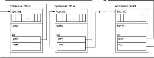

A further refinement of the linked list is an implementation where the head of the list has only a single pointer to the first element. This contrasts the double pointer head discussed in the previous section. Used in hash tables (which are introduced in Chapter 4, "Memory Management"), the single pointer head does not have a back pointer to reference the tail element of the list. This is thought to be less wasteful of memory because the tail pointer is not generally used in a hash search:

 ----------------------------------------------------------------------------- include/linux/list.h 484  struct hlist_head { 485   struct hlist_node *first; 486  }; 488  struct hlist_node { 489   struct hlist_node *next, **pprev; 490  }; 492  #define HLIST_HEAD_INIT { .first = NULL }  493  #define HLIST_HEAD(name) struct hlist_head name = { .first = NULL } ----------------------------------------------------------------------------- 

Line 492

The HLIST_HEAD_INIT macro sets the pointer first to the NULL pointer.

Line 493

The HLIST_HEAD macro creates the linked list by name and sets the pointer first to the NULL pointer.

These list constructs are used throughout the Linux kernel code in work queues, as we've seen in the scheduler, the timer, and the module-handling routines.

2.1.2. Searching

The previous section explored grouping elements in a list. An ordered list of elements is sorted based on a key value within each element (for example, each element having a key value greater than the previous element). If we want to find a particular element (based on its key), we start at the head and increment through the list, comparing the value of its key with the value we were searching for. If the value was not equal, we move on to the next element until we find the matching key. In this example, the time it takes to find a given element in the list is directly proportional to the value of the key. In other words, this linear search takes longer as more elements are added to the list.

Big-O

For a searching algorithm, big-O notation is the theoretical measure of the execution of an algorithm usually in time needed to find a given key. It represents the worst-case search time for a given number (n) elements. The big-O notation for a linear search is O(n/2), which indicates that, on average, half of the list is searched to find a given key.

Source: National Institute of Standards and Technology (www.nist.gov).

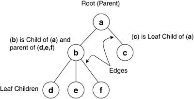
With large lists of elements, faster methods of storing and locating a given piece of data are required if the operating system is to be prevented from grinding to a halt. Although many methods (and their derivatives) exist, the other major data structure Linux uses for storage is the tree.

2.1.3. Trees

Used in Linux memory management, the tree allows for efficient access and manipulation of data. In this case, efficiency is measured in how fast we can store and retrieve a single piece of data among many. Basic trees, and specifically red black trees, are presented in this section and, for the specific Linux implementation and helper routines, see Chapter 6, "Filesystems." Rooted trees in computer science consist of nodes and edges (see Figure 2.3). The node represents the data element and the edges are the paths between the nodes. The first, or top, node in a rooted tree is the root node. Relationships between nodes are expressed as parent, child, and sibling, where each child has exactly one parent (except the root), each parent has one or more children, and siblings have the same parent. A node with no children is termed as a leaf. The height of a tree is the number of edges from the root to the most distant leaf. Each row of descendants across the tree is termed as a level. In Figure 2.3, b and c are one level below a, and d, e, and f are two levels below a. When looking at the data elements of a given set of siblings, ordered trees have the left-most sibling being the lowest value ascending in order to the right-most sibling. Trees are generally implemented as linked lists or arrays and the process of moving through a tree is called traversing the tree.

Figure 2.3. Rooted Tree

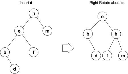
2.1.3.1. Binary Trees

Previously, we looked at finding a key using a linear search, comparing our key with each iteration. What if we could rule out half of the ordered list with every comparison?

A binary tree, unlike a linked list, is a hierarchical, rather than linear, data structure. In the binary tree, each element or node points to a left or right child node, and in turn, each child points to a left or right child, and so on. The main rule for ordering the nodes is that the child on the left has a key value less than the parent, and the child on the right has a value equal to or greater than the parent. As a result of this rule, we know that for a key value in a given node, the left child and all its descendants have a key value less than that given node and the right child and all its descendants have a key value greater than or equal to the given node.

When storing data in a binary tree, we reduce the amount of data to be searched by half during each iteration. In big-O notation, this yields a performance (with respect to the number of items searched) of O log(n). Compare this to the linear search big-O of O(n/2).

The algorithm used to traverse a binary tree is simple and hints of a recursive implementation because, at every node, we compare our key value and either descend left or right into the tree. The following is a discussion on the implementation, helper functions, and types of binary trees.

As just mentioned, a node in a binary tree can have one left child, one right child, a left and right child, or no children. The rule for an ordered binary tree is that for a given node value (x), the left child (and all its descendants) have values less than x and the right child (and all its descendants) have values greater than x. Following this rule, if an ordered set of values were inserted into a binary tree, it would end up being a linear list, resulting in a relatively slow linear search for a given value. For example, if we were to create a binary tree with the values [0,1,2,3,4,5,6], 0 would become the root; 1, being greater than 0, would become the right child; 2, being greater than 1, would become its right child; 3 would become the right child of 2; and so on.

A height-balanced binary tree is where no leaf is some number farther from the root than any other. As nodes are added to the binary tree, it needs to be rebalanced for efficient searching; this is accomplished through rotation. If, after an insertion, a given node (e), has a left child with descendants that are two levels greater than any other leaf, we must right-rotate node e. As shown in Figure 2.4, e becomes the parent of h, and the right child of e becomes the left child of h. If rebalancing is done after each insertion, we are guaranteed that we need at most one rotation. This rule of balance (no child shall have a leaf distance greater than one) is known as an AVL-tree (after G. M. Adelson-Velskii and E. M. Landis).

Figure 2.4. Right Rotation

2.1.3.2. Red Black Trees

The red black tree used in Linux memory management is similar to an AVL tree. A red black tree is a balanced binary tree in which each node has a red or black color attribute.

Here are the rules for a red black tree:

• All nodes are either red or black.

• If a node is red, both its children are black.

• All leaf nodes are black.

• When traversing from the root node to a leaf, each path contains the same number of black nodes.

Both AVL and red black trees have a big-O of O log(n), and depending on the data being inserted (sorted/unsorted) and searched, each can have their strong points. (Several papers on performance of binary search trees [BSTs] are readily available on the Web and make for interesting reading.)

As previously mentioned, many other data structures and associated search algorithms are used in computer science. This section's goal was to assist you in your exploration by introducing the concepts of the common structures used for organizing data in the Linux kernel. Having a basic understanding of the list and tree structures help you understand the more complex operations, such as memory management and queues, which are discussed in later chapters.