Multi-Area Configuration

The OSPF protocol supports the partitioning of a routing domain into multiple areas. The use of multiple areas will generally improve protocol scalability, as most link-state advertisement (LSA) types are not flooded across area boundaries. This means that a given router must only maintain a complete link-state database (LSDB) for the areas to which it actually connects. Distance vector-based routing is used between areas based on metrics that are carried in summary LSAs, which are generated by Area Border Routers (ABRs).

We begin our OSPF configuration example with the network topology shown in Figure 3.1.

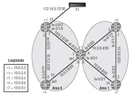
Figure 3.1: Multi-area OSPF

Referring to Figure 3.1, you can see that r5 will need to function as an ABR between the backbone (area 0) and transit area 1. To complete this configuration example, your OSPF configuration must meet the following criteria:

• Router ID (RID) based on lo0 address.

• lo0 address must be reachable via OSPF.

• Loopback addresses from backbone routers appear as summaries in area 1.

• The link between r3 and T1 must appear in area 0 as an intra-area route. Ensure that no adjacencies can be established on this interface.

r4 OSPF Configuration

We begin by configuring r4 as an internal backbone router with the following commands:

[edit protocols ospf] lab@r4# set area 0 interface lo0 passive [edit protocols ospf] lab@r4# set area 0 interface as0 [edit protocols ospf] lab@r4# set area 0 interface so-0/1/0.100 

These commands enable the main OSPF protocol instance, and place r4's lo0, its aggregated SONET interface as0, and its so-0/1/0.100 interfaces into area 0. By default JUNOS software will obtain the OSPF router ID from the first interface that is detected with a non-Martian address. Because lo0 is always the first interface examined when rpd starts, explicit configuration of the RID under routing-options is rarely necessary. Simply assigning the desired IP address to the lo0 interface results in a stable and deterministic router ID.

JUNOS software automatically advertises a stub route to the interface from which the RID is obtained; therefore it is not actually necessary to explicitly configure lo0 as an OSPF interface to meet the lo0 connectivity requirements of this configuration example.

Note 

Manually configuring the RID under routing-options will affect connectivity to the lo0 address, as the router will no longer include a stub route for its lo0 interface. You will have to enable OSPF on the lo0 interface, as done in the previous example, if lo0 connectivity is required and you have assigned the RID manually.

Omitting the lo0 interface from your OSPF configuration results in the lo0 address being advertised as a stub network in the router LSAs (type 1 LSAs) that are generated and flooded into all areas to which a given router attaches. Because your backbone routers must advertise their loopback addresses as a network summary route (LSA type 3) into the non-backbone areas, explicit association of the lo0 interface with the backbone area is required to meet the criteria of this example.

Because adjacencies cannot be formed on the router's lo0 interface, it has been configured to run as a passive interface in area 0. This prevents the unnecessary generation of hello packets and the general waste of compute cycles that would otherwise occur if lo0 were set as an active OSPF interface.

The resulting configuration for r4 is shown next:

[edit protocols ospf] lab@r4# show area 0.0.0.0 {    interface lo0.0 {       passive;    }    interface as0.0;    interface so-0/1/0.100;  }

It is worth noting that the correct logical interface has been specified for r4's so-0/1/0 interface. Omitting the logical unit number when specifying the interface name results in OSPF running on unit 0, which is the default logical unit number.

Verify OSPF on r4

After committing the initial OSPF configuration, we can display r4's OSPF interfaces to confirm proper backbone configuration. In the absence of other OSPF routers, we expect to find that r4 has no neighbors, and therefore, no adjacencies:

[edit protocols ospf] lab@r4# run show ospf interface Interface          State     Area         DR ID        BDR ID     Nbrs as0.0              PtToPt   0.0.0.0      0.0.0.0      0.0.0.0       0 lo0.0              DRother  0.0.0.0      0.0.0.0      0.0.0.0       0 so-0/1/0.100       PtToPt   0.0.0.0      0.0.0.0      0.0.0.0       0 

As predicted, r4 has no neighbors, but the display does indicate that the correct interfaces have been placed into area 0. To confirm that r4's lo0 address is reachable as an area 0 internal route, we display the contents of r4's router LSA:

[edit protocols ospf] lab@r4# run show ospf database detail    OSPF link state database, area 0.0.0.0  Type      ID          Adv Rtr        Seq      Age  Opt  Cksum Len Router *10.0.3.4     10.0.3.4    0x80000001    163  0x2  0x1bc4 60   bits 0x0, link count 3   id 10.0.2.8, data 255.255.255.252, type Stub (3)   TOS count 0, TOS 0 metric 1   id 10.0.3.4, data 255.255.255.255, type Stub (3)   TOS count 0, TOS 0 metric 0   id 10.0.2.4, data 255.255.255.252, type Stub (3)   TOS count 0, TOS 0 metric 1

As required, r4 is reporting its lo0 address as a stub link in its area 0 router LSA. We can also confirm that r4 has correctly obtained its RID from its lo0 address. You may need to restart routing to establish the correct RID, especially if the OSPF process was started before a non- Martian address was assigned to lo0.

r5 OSPF Configuration

The following commands define the correct interface and area associations needed by r5, which will function as an ABR:

[edit protocols ospf] lab@r5# set area 0 interface lo0 passive [edit protocols ospf] lab@r5# set area 0 interface at-0/2/1.35 [edit protocols ospf] lab@r5# set area 0 interface as1 

With all the area 0 interfaces specified, we now move on to area 1:

[edit protocols ospf] lab@r5# set area 1 interface fe-0/0/0 [edit protocols ospf] lab@r5# set area 1 interface fe-0/0/1 

The resulting multi-area configuration for r5 is shown next:

[edit protocols ospf] lab@r5# show area 0.0.0.0 {    interface lo0.0 {       passive;    }    interface at-0/2/1.35;    interface as1.0;  } area 0.0.0.1 {   interface fe-0/0/0.0;   interface fe-0/0/1.0;  }

Verify OSPF on r5

After committing r5's OSPF configuration, we expect to see an adjacency to r4, and the correct interface-to-area associations as indicated next:

[edit protocols ospf] lab@r5# run show ospf interface Interface        State       Area       DR ID      BDR ID     Nbrs as1.0            PtToPt     0.0.0.0    0.0.0.0     0.0.0.0      1 at-0/2/1.35      PtToPt     0.0.0.0    0.0.0.0     0.0.0.0      0 lo0.0            DRother    0.0.0.0    0.0.0.0     0.0.0.0      0 fe-0/0/0.0       DR         0.0.0.1    10.0.3.5    0.0.0.0      0 fe-0/0/1.0       DR         0.0.0.1    10.0.3.5    0.0.0.0      0 [edit protocols ospf] lab@r5# run show ospf neighbor   Address        Interface     State          ID         Pri    Dead 10.0.2.10       as1.0          Full          10.0.3.4     128    37 

These results confirm the presence of an OSPF adjacency between r4 and r5, and also confirm that the correct interface-to-area associations have been configured. Because r5 is an ABR, we can now examine a non-backbone area's link-state database to confirm that loopback addresses from backbone routers are being correctly injected into other areas as network summary LSAs:

[edit protocols ospf] lab@r5# run show ospf database netsummary area 1   OSPF link state database, area 0.0.0.1  Type        ID          Adv Rtr        Seq     Age  Opt  Cksum  Len Summary *10.0.2.0     10.0.3.5      0x80000001  489  0x2  0x3d04  28 Summary *10.0.2.4     10.0.3.5      0x80000001  489  0x2  0x1f1d  28 Summary *10.0.2.8     10.0.3.5      0x80000001  489  0x2  0xec4c  28 Summary *10.0.3.4     10.0.3.5      0x80000001  489  0x2  0x1C1d  28 Summary *10.0.3.5     10.0.3.5      0x80000001  489  0x2  0x831   28

This display indicates that r5 has generated several network summary LSAs for area 1, and that two of these summary LSAs are correctly reporting the loopback addresses of r4 and r5.

r3 OSPF Configuration

The following commands are entered on r3 to complete the configuration of the backbone area:

[edit protocols ospf] lab@r3# set area 0 interface fe-0/0/2 passive [edit protocols ospf] lab@r3# set area 0 interface lo0 passive [edit protocols ospf] lab@r3# set area 0 interface at-0/1/0.35 [edit protocols ospf] lab@r3# set area 0 interface so-0/2/0.100 

The configuration of r3 is now as follows:

[edit protocols ospf] lab@r3# show area 0.0.0.0 {   interface fe-0/0/2.0 {      passive;   }   interface lo0.0 {     passive;   }   interface at-0/1/0.35;   interface so-0/2/0.100;  }

By setting r3's fe-0/0/2 interface as passive, you ensure that no adjacencies can be formed over the interface and that the route to 172.16.0.12/30 will be injected into area 0 as an internal route. The passive setting on r3's fe-0/0/2 interface is needed to meet the requirements of this configuration example.

Verify OSPF on r3

With the backbone area configured, you expect to see that r3 has detected neighbors on both its at-0/1/0.35 and so-0/2/0.100 interfaces, and that the link to T1 is correctly reported in its router LSA:

lab@r3> show ospf interface Interface              State     Area            DR ID           BDR ID       Nbrs at-0/1/0.35            PtToPt   0.0.0.0         0.0.0.0         0.0.0.0         1 fe-0/0/2.0             DRother  0.0.0.0         0.0.0.0         0.0.0.0         0 lo0.0                  DRother  0.0.0.0         0.0.0.0         0.0.0.0         0 so-0/2/0.100           PtToPt   0.0.0.0         0.0.0.0         0.0.0.0         1 lab@r3> show ospf neighbor   Address         Interface             State      ID              Pri  Dead 10.0.2.1         at-0/1/0.35            Full      10.0.3.5         128    32 10.0.2.6         so-0/2/0.100           Full      10.0.3.4         128    35

These results confirm the correct interface and area settings are present in r3's OSPF configuration, and also verify that r3 has the expected adjacencies to r4 and r5. Next we will examine the contents of r3's router LSA to confirm the presence of the 172.16.0.12/30 prefix:

lab@r3> show ospf database router advertising-router 10.0.3.3 detail  OSPF link state database, area 0.0.0.0  Type ID Adv Rtr Seq Age Opt Cksum Len Router *10.0.3.3 10.0.3.3 0x80000003 103 0x2 0xbbf1 96  bits 0x0, link count 6  id 10.0.3.5, data 10.0.2.2, type PointToPoint (1)  TOS count 0, TOS 0 metric 1  id 10.0.2.0, data 255.255.255.252, type Stub (3)  TOS count 0, TOS 0 metric 1  id 172.16.0.12, data 255.255.255.252, type Stub (3)  TOS count 0, TOS 0 metric 1  id 10.0.3.3, data 255.255.255.255, type Stub (3)  TOS count 0, TOS 0 metric 0  id 10.0.3.4, data 10.0.2.5, type PointToPoint (1)  TOS count 0, TOS 0 metric 1  id 10.0.2.4, data 255.255.255.252, type Stub (3)  TOS count 0, TOS 0 metric 1

As expected, we see that the external link to T1 is being reported as an OSPF stub route, as shown with highlights.

Area 1 Configuration

The following commands correctly configure r6 for operation as an internal area 1 router:

[edit protocols ospf] lab@r6# set area 1 interface fe-0/1/0 [edit protocols ospf] lab@r6# set area 1 interface fe-0/1/1 

The specification of r6's lo0 interface is not necessary to meet the requirements of this example. The default JUNOS software behavior will result in r6 using the configured lo0 address as its RID, which in turn results in the automatic advertisement of this address as a stub route in r6's router LSA. The configuration of r7 is nearly identical to that of r6, with the only differences relating to interface-naming particulars. The configuration of r6 is shown next:

[edit protocols ospf] lab@r6# show area 0.0.0.1 {    interface fe-0/1/0.0;    interface fe-0/1/1.0;  }

Verify Overall OSPF Operation

The various spot checks performed thus far have all indicated the expected OSPF behavior and operation. This author has found that the following commands, which should be issued on an ABR, prove invaluable when the goal is to quickly assess the operational state of a multi-area OSPF configuration. The first command verifies that we have the expected number of router LSAs, which is 6 in this case, 3 in area 0, and 3 in area 1:

lab@r5> show ospf database router area 0     OSPF link state database, area 0.0.0.0  Type       ID               Adv Rtr           Seq       Age  Opt  Cksum  Len Router   10.0.3.3         10.0.3.3          0x80000003  1604  0x2  0xbbf1  96 Router   10.0.3.4         10.0.3.4          0x80000003  1611  0x2  0x373e  84 Router  *10.0.3.5         10.0.3.5         0x80000005    305  0x2  0x3446  84

As expected, three router LSAs have been flooded in area 0, one of which has been generated by r5 itself. The following confirms that area 1 also has the expected number of router LSAs:

lab@r5> show ospf database router area 1     OSPF link state database, area 0.0.0.1  Type       ID               Adv Rtr           Seq       Age  Opt  Cksum  Len Router  *10.0.3.5         10.0.3.5         0x80000008    374  0x2  0x9020  48 Router   10.0.9.6         10.0.9.6         0x80000005    337  0x2  0x5f2e  60 Router   10.0.9.7         10.0.9.7         0x80000004    338  0x2  0xa6db  60

The resulting display indicates that three routers currently belong to area 1, which is the expected result based on the topology being configured. It is interesting to note that r5 has generated two router LSAs, one that is flooded into area 0 and another that is flooded into area 1.

When dealing with a large number of routers, it will sometimes prove helpful to pipe the results of these types of commands to the CLI's match and count functionalities:

lab@r5> show ospf database router | match router | count Count: 6 lines

Considering that the ABR has generated two router LSAs, the five routers that make up this multi-area OSPF network is expected to produce a total of six router LSAs, so the results of this command indicate that all routers are present and that each router has at least one functional adjacency. Because the whole purpose of OSPF is to build a routing table, it might be wise to verify that the correct routing tables are being built as a result of all this LSA flooding. While the operator can always display the routing table and/or conduct ping testing to the various addresses that make up the test bed, this author has found it beneficial to perform spot checks such as the following, which quickly confirms that the loopback addresses of all remote routers are present as OSPF routes:

lab@r5> show route protocol ospf | match /32 10.0.3.3/32         *[OSPF/10] 00:35:19, metric 1 10.0.3.4/32         *[OSPF/10] 00:53:09, metric 1 10.0.9.6/32         *[OSPF/10] 00:15:07, metric 1 10.0.9.7/32         *[OSPF/10] 00:14:50, metric 1 224.0.0.5/32        *[OSPF/10] 00:53:14, metric 1

This display, taken from r5, confirms that the loopback addresses from the four remote routers are present as OSPF routes. r5's loopback address is not displayed here, because from r5's perspective, this address is not learned via OSPF. The 224.0.0.5/32 route is the ALL-OSPF router multicast address, and is always present as an OSPF route. Broken adjacencies are sure to cause grief during a lab-based examination, so you should verify the state of all adjacencies before considering your OSPF configuration complete. There are no shortcuts here. You will need to manually display and inspect the adjacency status on several of the routers that make up your JNCIP practice rack to verify the state of all adjacencies.

Tip 

Because it takes at least two routers to form an adjacency, there is no need to check every router in the test bed for adjacency status. By choosing wisely, one can minimize the number of routers that must be checked in order to confirm that all adjacencies are functional. For example, displaying the adjacency status on the DR (or BDR) will allow the quick confirmation of all adjacencies associated with a broadcast network.

We next display OSPF adjacency information from r3, r4, and r7, to verify the adjacency status of all five routers in the test bed:

lab@r3>  show ospf neighbor   Address         Interface             State      ID              Pri  Dead 10.0.2.1         at-0/1/0.35            Full      10.0.3.5         128   32 10.0.2.6         so-0/2/0.100           Full      10.0.3.4         128   35 lab@r5>  show ospf neighbor   Address         Interface             State      ID              Pri  Dead 10.0.2.10        as1.0                  Full      10.0.3.4         128    32 10.0.2.2         at-0/2/1.35            Full      10.0.3.3         128    31 10.0.8.5         fe-0/0/0.0             Full      10.0.9.6         128    35 lab@r7>  show ospf neighbor   Address         Interface             State      ID              Pri  Dead 10.0.8.1         fe-0/3/0.0             ExStart   10.0.9.6         128    35 10.0.8.9         fe-0/3/1.0             Full      10.0.3.5         128    32

While r3 and r5 show the proper adjacency counts and state, it would seem from these displays that there is a problem with the adjacency between r6 and r7.

Troubleshooting Adjacency Problems

Those experienced with OSPF adjacency formation and troubleshooting will recall that, after achieving two-way communications, OSPF neighbors wishing to form an adjacency will enter the state of 'Exchange Start' for the purpose of exchanging the contents of their LSDBs. After exchanging the database contents, and receiving acknowledgments from the remote router, the adjacency transitions to the full state. In this example, r6 and r7 are stuck at the exchange-start phase of adjacency formation. Because the exchange-start state confirms that both routers have successfully exchanged IP packets, there is little point in performing ping testing to fault isolate this type of problem.

One of the best ways to troubleshoot OSPF adjacency problems is to deploy tracing with special attention placed on hello packet exchanges, database descriptions, and any error messages that may be occurring. The following traceoptions configuration on r7 focuses on these message types:

lab@r7# show protocols ospf traceoptions file ospf; flag hello detail; flag error detail; flag database-description detail;

The result of monitoring the ospf trace file is shown next. To minimize clutter, r7 has its fe-0/3/1 interface disabled during the trace operation. The trace begins after the neighbor state is cleared:

lab@r7> clear ospf neighbor Apr 24 12:18:58 RPD_OSPF_NBRDOWN: OSPF neighbor 10.0.8.1 (fe-0/3/0.0) state  changed from Exchange to Down due to Kill all neighbors Apr 24 12:18:58 OSPF DR is 10.0.9.7, BDR is 0.0.0.0 Apr 24 12:18:59 OSPF sent Hello 10.0.8.2 -> 224.0.0.5 (fe-0/3/0.0) Apr 24 12:18:59    Version 2, length 44, ID 10.0.9.7, area 0.0.0.1 Apr 24 12:18:59    checksum 0xdC1c, authtype 0 Apr 24 12:18:59    mask 255.255.255.252, hello_ivl 10, opts 0x2, prio 128 Apr 24 12:18:59   dead_ivl 40, DR 10.0.8.2, BDR 0.0.0.0 Apr 24 12:19:00 OSPF rcvd Hello 10.0.8.1 -> 224.0.0.5 (fe-0/3/0.0) Apr 24 12:19:00    Version 2, length 48, ID 10.0.9.6, area 0.0.0.1 Apr 24 12:19:00    checksum 0xcf14, authtype 0 Apr 24 12:19:00    mask 255.255.255.252, hello_ivl 10, opts 0x2, prio 128 Apr 24 12:19:00   dead_ivl 40, DR 10.0.8.1, BDR 0.0.0.0 Apr 24 12:19:00 RPD_OSPF_NBRUP: OSPF neighbor 10.0.8.1 (fe-0/3/0.0) state  changed from Init to ExStart due to Two way communication established 

So far, all has been normal with the OSPF packet exchange and adjacency formation. The establishment of the two-way state confirms that the two routers agree on the area number, its type (transit in this case), logical IP subnet information, timer settings (hello and dead interval), etc. The trace output continues next, where we can see the exchange of database description messages:

 Apr 24 12:19:00 OSPF DR is 10.0.9.7, BDR is 10.0.9.6 Apr 24 12:19:00 OSPF sent DbD 10.0.8.2 -> 10.0.8.1 (fe-0/3/0.0) Apr 24 12:19:00   Version 2, length 32, ID 10.0.9.7, area 0.0.0.1 Apr 24 12:19:00   checksum 0x7790, authtype 0 Apr 24 12:19:00   options 0x42, i 1, m 1, ms 1, seq 0xa0f1da0, mtu 3986 

After correctly establishing their roles as master or slave for the database synchronization exchange, we next see 10.0.8.2 sending a database description packet to 10.0.8.1:

Apr 24 12:19:01 OSPF sent Hello 10.0.8.2 -> 224.0.0.5 (fe-0/3/0.0) Apr 24 12:19:01    Version 2, length 48, ID 10.0.9.7, area 0.0.0.1 Apr 24 12:19:01    checksum 0xbd12, authtype 0 Apr 24 12:19:01   mask 255.255.255.252, hello_ivl 10, opts 0x2, prio 128 Apr 24 12:19:01   dead_ivl 40, DR 10.0.8.1, BDR 10.0.8.2 Apr 24 12:19:01 OSPF rcvd DbD 10.0.8.1 -> 10.0.8.2 (fe-0/3/0.0) Apr 24 12:19:01    Version 2, length 32, ID 10.0.9.6, area 0.0.0.1 Apr 24 12:19:01    checksum 0x66a2, authtype 0 Apr 24 12:19:01   options 0x42, i 1, m 1, ms 1, seq 0xa0f3843, mtu 1500 Apr 24 12:19:01 OSPF now slave for nbr 10.0.8.1 . . .

After some hello exchanges, we next see r7 (10.0.8.2) receiving a database description packet from r6 (10.0.8.1). A short while later, the following trace output is observed:

. . . Apr 24 12:19:06 OSPF rcvd DbD 10.0.8.1 -> 10.0.8.2 (fe-0/3/0.0) Apr 24 12:19:06   Version 2, length 32, ID 10.0.9.6, area 0.0.0.1 Apr 24 12:19:06   checksum 0x66a2, authtype 0 Apr 24 12:19:06   options 0x42, i 1, m 1, ms 1, seq 0xa0f3843, mtu 1500 Apr 24 12:19:06   Duplicate Apr 24 12:19:06 OSPF resend last DBD to 10.0.8.1 

Though perhaps not obvious, the lack of database description acknowledgment, and the indication that duplicate database description packets are being sent, indicate that the two routers are discarding each other's database descriptions.

Because the majority of configuration problems (or bit errors) would prevent the establishment of two-way communications, this problem must relate to the nature of the database description packets themselves. Closer inspection of the trace output reveals that the database description packets sent by r7 have an IP layer MTU of 3986, while the packets sent by r6 indicate that the default MTU setting of 1500 bytes is in place. After correctly setting r6's fe-0/1/1 interface MTU to the correct value of 4000 as specified in the interface case study, the r6 to r7 adjacency can be correctly established:

lab@r7> show ospf neighbor   Address         Interface             State      ID              Pri  Dead 10.0.8.1         fe-0/3/0.0             Full      10.0.9.6         128    35 10.0.8.9         fe-0/3/1.0             Full      10.0.3.5         128    32

Now that all adjacencies have been confirmed, the initial OSPF multi-area configuration example can be considered a success!