Using Advanced AutoFilter Functions

In Hour 21, you learn about filtering data with Excel's nifty AutoFilter feature. This session takes that discussion one step further and talks about using advanced AutoFilter functions, such as extracting filtered data, and using the Top 10 AutoFilter and Custom AutoFilter options.

After you filter your records to display specific data in your database, you can extract that data by copying it to another worksheet or workbook. It's simple to dojust use the Copy and Paste tools to place the filtered data somewhere else.

As for fancy AutoFilter functions, you have Custom AutoFilter that lets you set up comparison criteria, as well as create AND or OR criteria. For example, you can search for all the employee ID numbers less than 650. An AND criteria could be filtering all employee ID numbers less than 650, and they must be in the Accounting department. An OR criteria could be filtering all employee ID numbers greater than 660 or employees who have worked more than 10 years for the company.

Perform the steps in the To Do exercise using the Top 10 and Custom AutoFilter features to display specific data in the My Database file.

To Do: Use Advanced AutoFilter Functions

1. Widen column F to accommodate the long column heading. Simply double-click the column border between columns F and G. Select any cell in the list. Now you've selected a cell within the list you want to filter.

2. Choose Data, Filter, AutoFilter. Excel displays drop-down arrow buttons next to each column heading in the database, as shown in Figure 22.5.

   Figure 22.5. AutoFilter arrow buttons next to the column headings.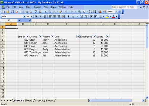

   

3. Click the drop-down arrow for the EmpPeriod column. The drop-down list shows the unique values for the column. Select Top 10. The Top 10 AutoFilter dialog box opens, as shown in Figure 22.6.

   Figure 22.6. The Top 10 AutoFilter dialog box.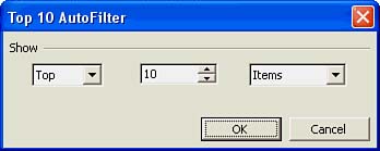

   

   

   You can click the column heading and press Alt+Down Arrow to see a drop-down list of data you want to display.

   
   

4. Change the number 10 to 4 and click OK to show the top four items. You should see four records, and the rest of the records are hidden. The blue arrow on the filter button indicates the filtered data is based on criteria you selected in the EmpPeriod column. The row header numbers for the filtered records also appear in blue.

5. To show all the records again, choose Data, Filter, Show All. Now you should see all six records so that Excel can filter records based on all the records in the entire database. Now you want to enter a custom filter to show all records with a salary greater than $40,000.

   

   When you choose Data, Filter, if a check mark appears next to the AutoFilter option, select AutoFilter to turn it off before selecting another Excel database.

   
   

6. Click the drop-down arrow for the Salary column. Choose Custom to open the Custom AutoFilter dialog box (see Figure 22.7).

   Figure 22.7. The Custom AutoFilter dialog box.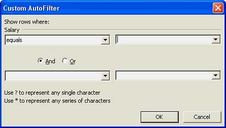

   

7. In the first Salary box on the left (it shows equals ), choose is greater than . In the second Salary box on the right, click the drop-down arrow and choose 40,000 . Click OK. You should see three records, and the rest of the records should be hidden.

8. Now that you are finished filtering, shut off AutoFilter. Choose Data, Filter, AutoFilter. This step removes the drop-down arrow buttons from the column headings in the database, redisplays the hidden rows, and turns off the AutoFilter feature for this database.