How to Use Lookup Functions

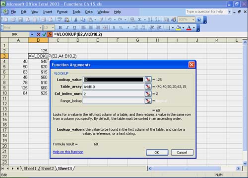
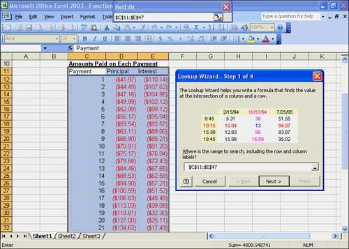
Lookup functions search for values within tables or lists. Each lookup function uses a different method for searching and returning values. Each method is suited for a particular task. Anytime your worksheet uses tables to hold values, such as tax tables or price tables, you can employ a lookup function for added power in the application.

VLOOKUP and HLOOKUP

These two lookup functions search for values in tables based on a lookup value, the value you are trying to match. For example, a tax table contains tax rates based on income. Income is the lookup value. VLOOKUP searches vertically in a column of values and then returns a corresponding value from the table. HLOOKUP searches horizontally in a row of values and then returns a corresponding value from the table.

If the lookup range within the specified table range contains text strings, the search variable must also be a text string. In such cases, the lookup function must be able to find an exact match for the specified information, including upper- and lowercase letters . If no match is found, the function returns the error #VALUE! . The data in the table (that is, the value to be returned) can be numeric values or text. The syntax for the HLOOKUP function is

 =HLOOKUP(value,range,row offset) 

As an example, suppose you have a table of prices for merchandise and want to search that table for item number 125 . When item number 125 is located in the table, the price of the item is returned.

The VLOOKUP function searches vertically in a column of values and then returns a corresponding value from another table column. The function works like this:

 =VLOOKUP(value,table range,offset) 

An example of a vertical lookup function is

 =VLOOKUP(B2,A4:B10,2) 

The value is the number or text in the first column of the table that you are trying to match with corresponding information. It can be any number, text, cell reference, or formula. For the Figure 15.10 example, the value was entered as the cell reference B2 so that any number entered into cell B2 becomes the value for the lookup. The table range is the worksheet range containing the table. The first column of this range, called the lookup column, should include the list of values for which you will be searching. The table can then include as many more columns as necessary to contain all information. Additional columns are called offset columns , and they contain the cells with information you want to return when you select a value from the lookup column. When entering the VLOOKUP formula, the lookup column is referred to as offset 1, the next column is offset 2, and so on.

Figure 15.10. Using the VLOOKUP function.

When the function finds the lookup value in the lookup column, it remembers the row position of the lookup value. Then the function searches across the table to return information from the column specified by the offset value listed in the formula. The lookup formulas in cells B3, C3, and D3 return information from each of the columns of the table, using the following functions:

 =VLOOKUP(B2,A4:D10,2) =VLOOKUP(B2,A4:D10,3) =VLOOKUP(B2,A4:D10,4) 

Notice that the formulas are almost identical; the only difference is that they contain different offset values, selecting values from different columns along one row of the table.

When you create lookup tables and the lookup formulas that use them, keep some basic rules in mind. First, the values in the lookup column must be in ascending order (sorted). If the values are text, they must be in alphabetical order. If the lookup column is not in ascending order, the function might return incorrect values. Excel searches the lookup column until it finds a direct match. If a direct match cannot be found, the closest value smaller than the search variable is used. Therefore, if a lookup value is greater than all values in the table, the last value in the table is used because it's the largest. If the lookup value is smaller than all values in the table, the function returns the error #VALUE! .

If the lookup column contains text, the lookup function must be able to match the lookup value exactly, including upper- and lowercase letters. When no match is found, the function returns the error #VALUE! . Even if the lookup column contains text, the offset columns can contain numeric values or text.

Lookup Wizard

Excel's Lookup Wizard can step you through searching for values in tables based on a lookup value, the value you are trying to find. As an example, if you have a price table that contains prices for merchandise based on item numbers , price is the lookup value. What if you want to search that table for item number 50? The Lookup Wizard searches vertically in a column of values and horizontally in a row of values, finds the value at the intersection of the column and row, and then returns that value from the table. For instance, the price of item number 50 is returned and copied into a cell on the worksheet.

Excel can copy the results in two ways:

• Copy just the lookup formula with its result into a cell.

• Copy the lookup formula with its lookup parameters (the column label, the row label, and the formula with its result).

The next exercise enables you to practice using the Lookup Wizard to find the interest on payment number 10. You'll be working with the Amounts Paid on Each Payment table in Sheet1 again.

To Do: Look Up a Value with the Lookup Wizard

1. Click the Sheet1 tab.

2. Select C11:E47, which is the range you want to search.

   

   Make sure you include the column and row headings in the range you select. The Lookup Wizard refers to column headings as column labels and row headings as row labels.

   
   

3. Click Tools in the menu and choose Lookup. The Lookup WizardStep 1 of 4 dialog box appears, as shown in Figure 15.11. You should see the selected range $C$11:$E$47 in the dialog box. This range is the one you want.

   Figure 15.11. The Lookup Wizard Step 1 of 4 dialog box.

   

   

   If the Lookup Wizard is not on your Tools menu, the add-in Lookup Wizard was not installed on your computer. To install the Lookup Wizard, choose Tools, Add-Ins. Scroll down the list until you see the Lookup Wizard and click its check box. Click OK. Excel displays instructions for installing the Lookup Wizard add-in from the Microsoft Office or Microsoft Excel CD-ROM.

   
   

4. Click the Next button. The Lookup WizardStep 2 of 4 dialog box pops up.

5. In the Which Column Contains the Value to Find box, choose Interest. This step selects the column label.

6. In the Which Row Contains the Value to Find box, choose Payment. This step selects the row label.

7. Click the Next button. The Lookup WizardStep 3 of 4 dialog box shows up. The Copy Just the Formula to a Single Cell option should be selected. You want this option. You should also see the return value of E21 , which is the item number that the Lookup Wizard found in the table.

8. Click the Next button. The Lookup WizardStep 4 of 4 dialog box should appear.

9. Click cell C52. This step tells Excel where to copy the formula.

10. Click the Finish button. Excel shows the result $81.20 in cell C52.