Protecting Your Data

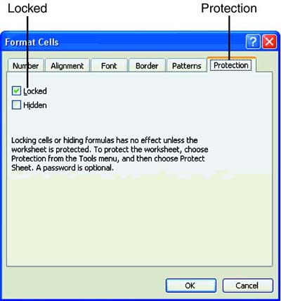
If a worksheet contains cells you do not want changed, you can lock them so that they cannot be edited or deleted. You can also add a password to a sheet or workbook to protect the entire sheet or workbook.

If you have columns and rows that you do not want anyone to see or change, you can hide the columns and rows and then display them again whenever you wish.

Locking Cells

To set cell protection, perform the steps in the To Do exercise. You want to lock all the cells in your worksheet except for the numbers for March in column D.

To Do: Lock Cells

1. In the Summary sheet, select cells D4:D8. You want to protect these cells from being locked.

2. Choose Format, Cells. The Format Cells dialog box appears.

3. Click the Protection tab, as shown in Figure 14.19. A check mark appears in the Locked check box, which means that all cells are locked.

   Figure 14.19. The Protection tab in the Format Cells dialog box.

   

4. Click the Locked check box. This step removes the check mark, which indicates the selected cells will not be locked.

5. Click OK.

6. Click any cell in column C and type anything. Excel permits you to do so because the worksheet is not protected from changes. For cell or object protection to be in effect, you must turn on worksheet protection. You will learn how to do this in the next section.

7. Click the Undo button on the Standard toolbar to reverse the change.

For cell or object protection to be in effect, you must turn on worksheet protection.

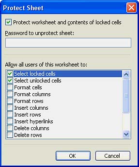
Protecting a Worksheet

By default, cells are locked, but the worksheet protection is not on. You can unlock all the cells you want to change and then turn on worksheet protection.

To protect the worksheet, choose Tools, Protection, Protect Sheet. Excel displays the Protect Sheet dialog box, as shown in Figure 14.20.

Figure 14.20. The Protect Sheet dialog box.

You can protect the sheet for selecting, formatting, inserting, deleting, sorting, AutoFilter, PivotTable reports , objects, and scenarios. By default, the worksheet and contents of locked cells is protected, along with the act of selecting locked and unlocked cells is protected. A password is optional. Choose OK to protect the worksheet.

Now, to test whether the cells are locked, click cell C4, type 950 , and press Enter. Notice that when you try to edit locked cells, an alert box tells you that locked cells cannot be changed. Choose OK to clear the alert box. Excel prevents you from making the change to the cell because the cell is locked and the worksheet is protected.

Now try to type a number in cell D4. Can you do it? The answer should be yes. Excel allows you to type in a cell that is not locked.

To turn off worksheet protection, choose Tools, Protection, Unprotect sheet.

Protecting the Workbook

You might want to protect the structure of a workbook and the windows . Here are the structure elements you can protect in a workbook:

• Viewing hidden worksheets.

• Changing the names of worksheets.

• Moving, deleting, hiding, or worksheets.

• Inserting new worksheets or chart sheets. You can add an embedded chart to an existing worksheet with the Chart Wizard.

• Moving or copying worksheets to another workbook.

• In a PivotTable report, displaying the source data for a cell in the data area, or displaying page field pages on separate worksheets.

• Creating a scenario summary report.

• Using the analysis tools in the Analysis ToolPak that inserts results on a new worksheet.

• Recording new macros.

Here are the windows elements you can protect in a workbook:

• Changing the size and position of the windows.

• Moving, resizing, or closing the windows.

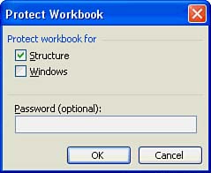
You can assign a password (optional) so that users need a password to change the structure of, or windows in, the workbook.

To protect a workbook, click Tools in the menu bar and choose Protection, Protect Workbook. Excel opens the Protect Workbook dialog box, as shown in Figure 14.21.

Figure 14.21. The Protect Workbook dialog box.

To select the elements you want to protect, click in the Structure check box to protect the worksheets in the workbook. Click in the Windows check box so that the size and position of the windows cannot be changed. If you want, type a password in the Password box, click OK, and type the password again. Click OK.

When you want to unprotect the workbook, choose Tools, Protection, Unprotect Workbook. The Unprotect Workbook dialog box opens. Enter the password and then click OK. Your workbook is now unprotected .

Remember your password. If you forget it, you cannot unprotect your workbook. Also, passwords must be entered in the exact upper- and/or lowercase letters .

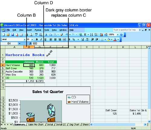
Hiding and Displaying Rows and Columns

A worksheet might contain columns and rows that you don't want to appear on the worksheet. If so, you can easily hide columns and rows with the Hide command or with the mouse. Remember that hidden elements don't print when you print the worksheet.

To use the Hide command to hide columns, select the column you want to hide by clicking the column header (the column header contains the column letter). You can hide additional columns by pressing the Ctrl key while clicking each column header. Then choose Format, Column, Hide. If you hide column C, for example, only columns A, B, D, E, and so on are visible (see Figure 14.22). A dark gray border between columns B and D replaces column C in the column header.

Figure 14.22. Column C is hidden.

To display hidden columns, highlight the two columns on either side of the hidden column. For instance, if column C is hidden, highlight columns B and D. Choose Format, Column, Unhide. Excel displays the hidden column.

Here's how you can use the mouse to hide and unhide columns:

• To use the mouse to hide a column, point to the column's right border. Drag the right column border past the left column border. The column disappears.

• To unhide a column with the mouse, point to the left border of the column heading to the right of the hidden column. For example, if column C is hidden, point to the left border of column heading D. When the mouse pointer border turns into a double-lined border, drag the column border to the right.

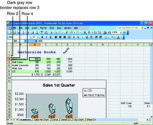
To use the Hide command to hide rows, select the row you want to hide by clicking the row header (the row header contains the row number). After selecting one row, you can select other rows by pressing the Ctrl key while clicking each row header. Then choose Format, Row, Hide. If you hide row 3, for example, only rows 1, 2, 4, 5, and so on are visible. A dark gray border replaces the hidden row in the row header (see Figure 14.23).

Figure 14.23. Row 3 is hidden.

To display hidden rows, highlight the rows above and below the hidden row. For instance, if row 3 is hidden, highlight rows 2 and 4. Choose Format, Row, Unhide. Excel displays the hidden row.

Here's how to use the mouse to hide and unhide rows:

• To use the mouse to hide a row, point to the row header's bottom border. Drag the bottom row border past the top row border. The row disappears.

• To unhide a row with the mouse, point to the dark gray borderline between two row headings next to the hidden row. For example, if row 3 is hidden, point to the dark gray borderline between row headings 2 and 4. Move the mouse down slightly until you have a double-lined border mouse pointer and then drag the row border down. The hidden row appears.