Policy-Based Network Management (PBNM)
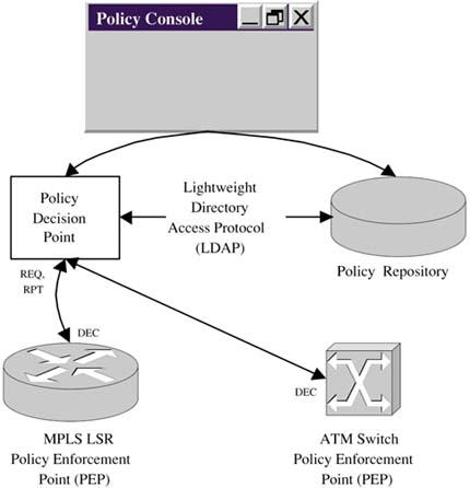
| PBNM is one of the most important directions being taken in network management. It recognizes that trying to manage individual devices and connections using a simple get/set/notification model is no longer sufficient because of the demands increasingly being placed on networks. Devices must become a lot more self-reliant in allowing the network operator to divide up and control the underlying resources in a deterministic fashion. PBNM introduces a number of new and interesting entities into network management, as shown in Figure 4-5, which illustrates the main PBNM architectural elements:
Figure 4-5. PBNM architecture. Policy consoles are employed to manage user-generated policies. The user creates, deletes, and modifies policies, and these are saved into the repository. The PDP or policy server is responsible for pushing (or installing) policies onto the various NEs. PEPs are NEs (such as IP routers, switches, or MPLS nodes) that execute policies against network resources like IP traffic. Policies can be installed by the PDP without any prompting from PEPs; alternatively, PEPs may initiate requests to the PDP to download device-specific policies; for example, if the PEP is an MPLS node, then it can download traffic engineering policies. The architecture in Figure 4-5 is flexible enough to support both modes of operation. The PDP retrieves policies from the repository using the Lightweight Directory Access Protocol (LDAP). COPS-PR is the protocol used to move policy configuration from a PDP to a PEP. A simple protocol is used for policy manipulation by PEPs consisting of these messages: REQ (uest), DEC (ision), and RPT (report) ”as illustrated in Figure 4-5. The PBNM elements in Figure 4-5 form an adjunct to (not a replacement for) the NMS we have discussed so far. Policies installed on NEs provide a very fine-grained control mechanism for network operators. What Is a Policy? ”Pushing Intelligence into the NetworkPolicies add intelligence to NEs; in effect, the network becomes almost like a computer, performing advanced functions with no further prompting needed from an external NMS. Policies are simply rules that contain essentially two components :
Policies are in widespread use in computing. A simple example is that of IP router table control. A network of IP routers is a dynamic entity because nodes and links in the network can go up and down, potentially resulting in changes to the paths taken by traffic. All of the routers try to maintain a current picture of the network topology ”similar to the way an NMS tries to maintain a picture of its managed objects. Figure 4-6 illustrates an autonomous system (AS) comprised of four interior (intra-AS) routers and two exterior (inter-AS) routers. A real AS could contain hundreds or thousands of nodes. Figure 4-6. An IP autonomous system. The interrouter links in Figure 4-6 are A, B, C, D, E, F, G, and H respectively, with administrative weights shown in brackets. Each router records those IP addresses reachable from itself in an optimal (in this case, least-cost) fashion; for example, the cheapest route from 10.81.1.2 to 10.81.1.6 is via links D and G respectively. Table 4-1 illustrates a conceptual extract from the routing table on 10.81.1.2. The clever way routers manage traffic is that they simply push it to the next hop along the path . In this case, 10.81.1.2 has a packet destined for 10.81.1.6, so the packet is sent to 10.81.1.3. Once this occurs, 10.81.1.2 forgets about the packet and moves on to its next packet. When 10.81.1.3 receives the packet, it also pushes the packet to the next hop indicated in its routing table (in this case the destination 10.81.1.6). By operating in this way, IP routers distribute the intelligence required to move packets to their destinations. Table 4-1. IP Routing Table for Router 10.81.1.2
The next hop for a packet, destined for 10.81.1.6, at router 10.81.1.2 is illustrated in Table 4-1 as 10.81.1.3. The administrative weight (or cost) of getting a packet from 10.81.1.2 to 10.81.1.6 is the sum of the intermediate link weights; this is the sum of link weights for D and G, or 4. When a change occurs in the network topology, the routers detect this and initiate a process called convergence. If link D in Figure 4-6 fails, then the shortest path to 10.81.1.6 (from 10.81.1.2) is recalculated to yield B-F-H. Table 4-1 would then be updated so that the next hop in the direction of 10.81.1.6 is 10.81.1.4 with a cost of 8. It is actually the interface that leads to 10.81.1.6. A number of steps precede this:
This is the way in which the routers update their picture of the network. Routing information exchanges can also be encrypted, though many core Internet routers do not employ this facility, which leaves them open to attacks [CERTWeb]. The Routing Policy Specification Language [RFC2622] provides a specification for this. Our discussion of IP routing has left out some important details. Figure 4-7 illustrates an extract from the route table for a Windows 2000 host with the IP address 10.82.211.29. To see this on a Windows machine, just open a DOS command prompt and type netstat “r . Figure 4-7 Host routing table. C:\>netstat -r Route Table ========================================================================= Active Routes: Network Destination Netmask Gateway Interface Metric 0.0.0.0 0.0.0.0 10.82.211.1 10.82.211.29 1 127.0.0.0 255.0.0.0 127.0.0.1 127.0.0.1 1 10.82.211.0 255.255.255.0 10.82.211.29 10.82.211.29 1 10.82.211.29 255.255.255.255 127.0.0.1 127.0.0.1 1 10.82.255.255 255.255.255.255 10.82.211.29 10.82.211.29 1 Default Gateway: 10.82.211.1 ========================================================================= Figure 4-7 illustrates a number of interesting features:
From all this we can see that a route table is just a set of rules for how to handle IP packets with specific destination addresses. This is the context we use for explaining policy [2] here.
To illustrate the way IP routing works, let's try using the ping command, ping 10.82.211.29 , to produce the listing illustrated in Figure 4-8. Ping is an application layer entity that sends an ICMP (another protocol in the TCP/IP suite) request packet to the specified host. Ping is very useful for determining if a given node is IP-reachable because when the ICMP request is received, a host must send a response similar to that in the listing. Let's now trace the message exchange. Figure 4-8 ICMP request and reply messages.C:\>ping 10.82.211.29 Pinging 10.82.211.29 with 32 bytes of data: Reply from 10.82.211.29: bytes=32 time<10ms TTL=128 Reply from 10.82.211.29: bytes=32 time<10ms TTL=128 Reply from 10.82.211.29: bytes=32 time<10ms TTL=128 Reply from 10.82.211.29: bytes=32 time<10ms TTL=128 Ping statistics for 10.82.211.29: Packets: Sent = 4, Received = 4, Lost = 0 (0% loss), Approximate round trip times in milli-seconds: Minimum = 0ms, Maximum = 0ms, Average = 0ms When the ICMP request packet arrives at the host (10.82.211.29), the route table is searched for the longest match. This is row four in Figure 4-7, shown in bold. The packet is relayed to the loopback interface 127.0.0.1 ”this has the effect of sending the packet back to the local host (we will see the loopback interface again in Chapter 7, "Rudimentary NMS Software Components," Figure 7-9). The local host then responds to the ping request with four packets. Other interesting information on the various TCP/IP protocols can be gleaned using related DOS commands such as arp and tracert . Appendix B, "Some Simple IP Routing Experiments," has some details. |
EAN: 2147483647
Pages: 150