Working with Mining Models
| < Day Day Up > |
Building a Mining ModelNow that the database has been created and populated, the next step is to create a mining model. Mining models can be created with the Mining Model Editor in Analysis Manager or programmatically with Decision Support Objects (DSO). Using DSO to create mining models is useful when you need to programmatically automate the mining-model process. For the most part, you will use Analysis Manager to create mining models. Analysis Manager (see Figure 5.3) allows you to create and manage databases used by Analysis Services. A database node in Analysis Manager does not represent the physical storage of a large database. Instead, it represents the database that Analysis Services will use to hold the mining-model definitions and the results of processing these mining models. It will, however, reference a physical data source. Figure 5.3. Screenshot of Analysis Manager, the utility used to create and manage mining models with Analysis Services. The Data Link Properties dialog box, used to specify the data source, is visible.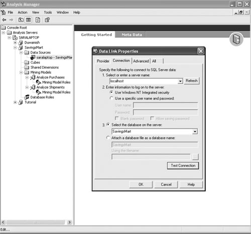 Each database in Analysis Manager is associated with one or more data sources. These data sources can be either relational databases or data warehouses. Data sources are created by right-clicking the Data Sources node and selecting New Data Source. From the Data Link Properties dialog, a data provider is selected along with the connection information. Analysis Services supports SQL Server, Access, and Oracle databases as data sources. Mining models are the blueprint for how the data should be analyzed or processed. Each model represents a case set, or a set of cases (see Table 5.1). The mining-model object stores the information necessary to process the model for instance, what queries are needed to get the data fields, what data fields are input columns or predictable columns, and what relationship each column has with other columns. Input columns are attributes whose values will be used to generate results for the predictable columns. In some cases, the attribute may serve both as an input column and a predictable column. Once the model is processed, the data associated with the mining model represents what was learned from the data. The actual data from the training dataset is not stored in the Analysis Services database. The results of analyzing that data, however, are saved. To quickly demonstrate the process of creating these models, we will walk through the process of creating a mining model using Analysis Manager. Tip If you have not already done so, you will need to install Analysis Services. It is available as a separate install with the SQL Server 2000 setup. Make sure that you install the latest Service Pack release for SQL Server. Information about how to obtain the latest SQL Server service pack can be found at http://support.microsoft.com/default.aspx?kbid=290211. If you have problems connecting with Analysis Services, refer to the article by Alexander Chigrik titled, "Troubleshooting OLAP Problems" at http://databasejournal.com/features/mssql/article.php/1582491. This online article, featured in the Database Journal, is a troubleshooting checklist for solving common problems. To begin, open Analysis Manager from the Analysis Services menu item. You will then need to create a new database and specify the data source by executing the following steps:
The next thing to do is create the mining model using the mining-model wizard. To do so, execute the following steps:
Note Choosing discretized as the content type allows a continuous variable to be grouped discretely instead. Continuous variables are usually numeric-based values that have an infinite range of possibilities. Since we need predictable results, utilizing a discretization method allows for grouped results. DISCRETEIZED accepts two parameters, such as:
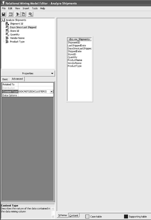
where method could contain one of the following values:
Training the Mining ModelTraining the mining model is accomplished by processing the results of a mining model using Analysis Manager. Alternatively, the same thing could be accomplished using a scripting language known as Data Definition Language (DDL) and a connection to the Analysis Server. We can see what DDL commands are used to train the model through the Process dialog box, as shown in Figure 5.5. Figure 5.5. Screenshot of the dialog that appears when full process is initiated for a mining model. Note the DDL syntax used to create the model and then train it by populating it with historical data.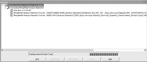 DDL is useful in cases when you want to programmatically process a mining model. The language can be executed through a connection to the Analysis Server. It is also useful for demonstrating how Analysis Manager processes a mining model. A mining model is created using the CREATE MINING MODEL syntax. The syntax is similar to Transact SQL and should be instantly familiar to SQL developers. The CREATE statement for this mining model is as follows: CREATE MINING MODEL [Analyze Shipments]( [Shipment Id] LONG KEY, [Days Since Last Shipped] LONG DISCRETIZED(CLUSTERS) PREDICT, [Store Id] LONG DISCRETE, [Quantity] LONG DISCRETIZED(CLUSTERS) PREDICT_ONLY, [Vendor Name] TEXT DISCRETE, [Product Type] TEXT DISCRETE) USING Microsoft_Decision_Trees With the preceding statement, we are creating a new mining model named Analyze Shipments. The model utilizes Shipment ID as the case key. Days Since Last Shipped, and Quantity are each defined as predictable columns, but Days Since Last Shipped also functions as an input column. The remaining columns, Store ID, Vendor Name, and Product Type, are input columns only. Mining-model columns are defined as either input, predictable, or input and predictable. The process of training a model involves the insertion of data into the mining model using the INSERT INTO syntax, as follows: INSERT INTO [Analyze Shipments] (SKIP,[Days Since Last Shipped], [Store Id], [Quantity], [Vendor Name], [Product Type]) OPENROWSET('SQLOLEDB.1','Provider=SQLOLEDB.1;Integrated Security=SSPI;Persist Security Info=False;Initial Catalog=SavingsMart;Data Source=(local)', 'SELECT DISTINCT "dbo"."vw_Shipments"."ShipmentID" AS "Shipment Id", "dbo"."vw_Shipments"."DaysSinceLastShipped" AS "Days Since Last Shipped", "dbo"."vw_Shipments"."StoreID" AS "Store Id", "dbo"."vw_Shipments"."Quantity" AS "Quantity", "dbo"."vw_Shipments"."VendorName" AS "Vendor Name", "dbo"."vw_Shipments"."ProductType" AS "Product Type" FROM "dbo"."vw_Shipments"') The mining model will not store the actual data, but will store the prediction results instead once the mining algorithm is processed. In the preceding statement, the OPENROWSET keyword was used to specify the location of the physical data source. Interpreting the ResultsTo examine the results from processing the model, select the Content tab. Figure 5.6 is a screenshot of the content detail when analyzing DaysSinceLastShipped. This screen indicates that VendorName was the most significant factor affecting DaysSinceLastShipped. We know this because it is the first split on the tree. For nodes that have additional branches, two lines will follow the node. To view the additional branches, double-click that node and the detail page will drill down to the next level. Figure 5.6. Screenshot of the content detail after processing the Analyze Shipments mining model. These results indicate the highest prediction level for the DaysSinceLastShipped column.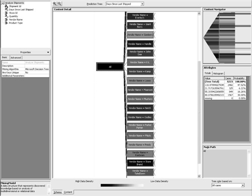 The Content Navigator box seen in the top-right corner offers an easy way to see all the mining-model results and drill down into a certain path. The Attributes box shows the totals associated with each node, grouped according to a clustering algorithm. In Figure 5.6, the cursor is selecting the outermost node labeled All. In this example, the attributes are shown for all the cases analyzed. Note If you did not attach the database file and instead loaded the data using the LoadSampleData program, you will encounter slightly different statistical results. The results presented in this section are specific to the database file available on the book's Web site. If you attached your database using the file provided, your processing results should be the same as the ones we are about to interpret. The first thing to notice is that the darkest-shaded node is the one where the Vendor Name is Store Brand. Nodes that resulted in a higher data density, or more cases analyzed, will be shaded in a darker color. This result is not surprising, because 127 of the 500 products available, or 25 percent, are represented by the Store Brand. This can be confirmed in Query Analyzer with the following query: SELECT v.VendorName,(COUNT(ProductID)/500.0) AS 'Percent' FROM Products p LEFT JOIN Vendors v ON p.VendorID = v.VendorID GROUP BY v.VendorName ORDER BY 'Percent' DESC If the Store Brand node is double-clicked, the detail pane will show the next branching of the tree (see Figure 5.7). For the Store Brand Node, the first branching distinguishes between the different stores. If we click on the node Store ID = 2 and look at the attributes, the value with the highest probability is 119.33. This indicates that for all products where the Vendor name is Store Brand and the Store ID is 2, it is highly probable that there should be 119 days between shipments. Figure 5.7. Screenshot of the Content Detail Editor as it displays the predictions for days since last shipped. In this example, the node path is where Store ID is 2 and the vendor name is Store Brand.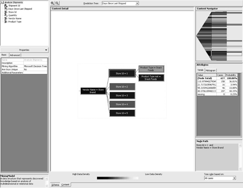 If we examine the attributes for the remaining nodes, we will see that predictions can be made for all the stores. For Store 1, there is one additional branching that distinguishes between a product type of Snack Foods versus all other product types. When the Store ID is 1, vendor name is Store Brand, and product type is snack foods, there is a 58 percent probability that there will be 60 days between shipments. When we examine the attributes where product type is not snack foods, there is a 43 percent probability that there will be 119 days between shipments and a 53 percent probability that there will be 85 days between shipments. In this case, we could say that the 53 percent probability wins the toss, but that might not always be the best decision. This will be discussed further in the next chapter. If you use the drop-down box above the Content Detail pane named Prediction Tree to select the quantity column, you will see that the main factor affecting quantity is the days since last shipped (see Figure 5.8). This is possible because the column DaysSinceLastShipped was defined as an input and a predictable column. Figure 5.8. Screenshot of the Content Detail Editor as it displays the predictions for Quantity. In this example, the node path examined is where Days Since Last Shipped is less than or equal to 48 and Store ID is not equal to 1 and vendor name is not equal to Kamp.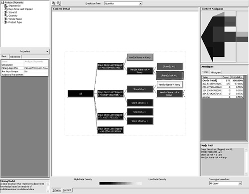 The next factor affecting quantity is the vendor name. In the case where the vendor name is NOT Kamp, Store ID is an additional factor. In Figure 5.8 we can see that when the days since last shipped is less than or equal to 48 and the Store ID is NOT 1 and the vendor name is NOT Kamp, there is a 98 percent probability that the quantity should be 200. When the Store ID is equal to 1, the prediction drops to a 72 percent probability that the quantity will be 200. The next chapter will involve interpreting the results from the mining model and then applying the predictions to a new shipment strategy. The goal of the new shipment strategy will be to reduce Savings Mart's operational costs by reducing the total number of shipments. |
| < Day Day Up > |
EAN: N/A
Pages: 123