Using Analysis Services Tools to Address Business Scenarios
| The following section discusses various scenarios and technical situations in which you may find yourself. The goal of presenting these scenarios is to go beyond the basic step-by-step of how to use the designers or wizards, but to actually provide tips on and insights into some non-obvious capabilities of the designers and wizards. To facilitate your search through these 30+ scenarios, I have categorized them each by the designers and wizards where they take place. Beyond this grouping they are not ordered in any particular way.
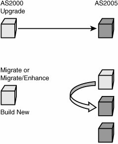
In the following sections we address each of these questions. How Should I Upgrade My Existing Application?This is one of the very first questions you may face. The answer is not that obvious because it depends on your business requirements, resources, and infrastructure. You have four main options:
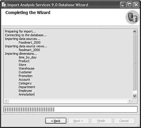
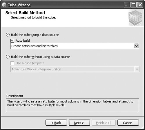
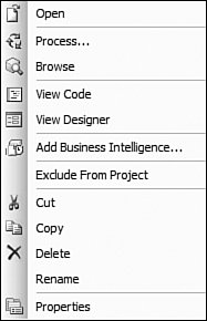
Let's look at each of these options in detail and evaluate their pros and cons. But before that, let's look at what your cube's situation would look like before and after you have installed Analysis Services 2005 and applied each of these techniques. Figure 13-13 illustrates what version of the software would be running on your server before and after an Upgrade, migration, or building a brand new cube. Each option is discussed in detail in the following sections. Figure 13-13. Upgrade and migration options. UpgradeUpgrade means the database and cube are upgraded from an AS200 to an AS2005 server in the same machine. After the upgrade the AS2000 server and cubes are no longer available, so there is no going back! Personally I would rarely recommend using the upgrade scenario. The main reason for this is that during an upgrade the cube is moved from an AS2000 to an AS2005 server on the same machine. Because the AS2000 cubes and DB are not available any longer, it is impossible to test after the upgrade and verify that the upgraded cubes return the same results as the cubes in AS2000. If you decide to upgrade we strongly, no, we STRONGLY recommend that you use the Upgrade Advisor utility before running the upgrade. The Upgrade Advisor can either be downloaded from Microsoft.com or installed from the SQL 2005 setup disk. The Upgrade Advisor provides you with a warning about potential areas affected during the upgrade and information about how to fix some of these issues. Also, you need to realize that after an upgrade, the AS database and cubes in AS2005 are an exact (as much as possible) image of the AS2000 database and cube, and thus they don't take advantage of any of the new architecture and features available in AS2005. Also be aware than an upgrade upgrades only the metadata, which means the cube and database need to be processed after the upgrade step. MigrateThe migration scenario is different than the upgrade scenario in the sense that SQL 2005 is installed side by side with SQL 2000. Although this requires more space on the server, it also provides you with a major benefit over upgrading. This benefit is the fact that after you migrate your AS database to AS2005, the AS2000 Database is still available. Thus both databases can be compared, and, if necessary, the AS2000 database can serve as a reference in case some modification needs to be applied to the newly migrated AS2005 database. During the migration, the migration wizard provides warnings and information similar to that delivered through the upgrade advisor. As in the upgrade scenario, the migration migrates only the metadata, so this means that the cubes and dimensions need to be reprocessed. As in the upgrade scenario, after a migration, the cube and database are an image of the AS2000 cube and database. Thus they don't take advantage of any of the new AS2005 functionality. Migrate and EnhanceMigrating and enhancing is a slight variation on the migration scenario. Indeed, after a migration the cubes and database are an image of the AS2000 cubes and database. But it is possible to enhance this design to start taking more advantage of the new functionality offered by AS 2005. The first thing that you want to take advantage of is the new project mode. Working in live mode against the server to modify and develop functionality can work only in situations or companies that do not have a lot of resources and specifically do not have different teams and people in charge of developing and managing the server. Moving off live mode to the project mode is important because it gives you a lot of possibilities. For one, you can now track versions of the cubes designs by using a source control system. Additionally multiple developers can now work on the project at the same time. And finally, your developers can update the design of the cubes and dimensions without impacting the users using the cubes and database. You can reverse-engineer the live database to an Analysis Services project by using the Import Analysis Services 9.0 database. Choose File> New Project (see Figure 13-14). Figure 13-14. Using the Import Analysis Services 9.0 database project.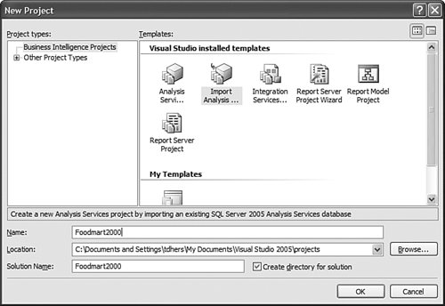 After you create the project, the Import Analysis Services 9.0 database wizard is launched (see Figure 13-15). You will notice that as an object gets read from the server and imported, the corresponding object is created on the fly in the Solution Explorer. Figure 13-15. Import an Analysis Services 9.0 Database Wizard. After the live database has been moved to a project, then the rest of the cube's design can be enhanced. For example, KPI can be added to the cube, additional hierarchies can be added to each dimension, or translations can be added to both dimension and cube objects. RebuildSometime, it may be better to spend a little more time early on when moving the database to Analysis Services 2005, if this provides a longer life to the application. It may indeed be better in some cases for you to rebuild existing applications using the new tools provided by AS2005, such as the Cube Wizard and its intelli-cube technology (see Figure 13-16). Figure 13-16. Using the Cube Wizard to automatically build a cube based on a data source. Note Intellicube is not the official name of this functionality. It is now called Autobuild. Interestingly, when Cristian Petculescu, our architect, first started working on this functionality, we called it the One Click cube. That was the result of the challenge that Amir Netz, our Product Unit manager, gave to Cristian. Wouldn't it be cool if we could build the entire cube and dimension automatically in one click. We still used this name internally when we referred to this feature, but we knew it wouldn't be the final one. When it came time to name this feature, the product group recommended Intellicube, because we are indeed trying to do our best and be as smart as possible in creating the best cube possible. The marketing and branding group came back with this new name which is now the official one: Auto Build. But for us, it is still the Intellicube feature powered by the One Click Cube algorithm. Anyway, building the cube from scratch may be a slightly lengthier process and a bigger investment in time and resources than upgrading or migrating an existing cube, but it has many advantages. First, your cube will be fully optimized for the new architecture that AS2005 offers. It will take full advantage of the new attribute-based architecture. The new cube will provide greater analytic capability: more and finer-grain data, more hierarchies, more measures coming from multiple measure groups, and more calculations. In conclusion, for this scenario, we offer you options. Don't jump into upgrading everything right away. Take a little time to assess your situation and decide whether it is worth investing some time rebuilding everything or whether things are just fine the way they are. If your cube provides you what you need (as we like to put it, "if it ain't broken, don't fix it"), then migration may be just fine. What Exactly Is the UDM?When I do Executive Briefing Center sessions (EBCS) or events like Teched, this is actually one of the most frequently asked questions: What exactly is a Unified Dimensional Model (UDM)? The UDM is the 2005 version of an Analysis Services cube. It is a cube! One could also wonder, then why did we call that a UDM? It is a cube indeed, but not a cube like the one you may be used to seeing with AS2000 or with other vendor technology. It goes much beyond what people think of traditionally as a cube. A UDM is a technology that enables you to model all the data contained in your data source(s), not just simple hierarchies. It also contains all the attributes (mapping to columns in the tables) available. Beyond potentially providing the same level of detail as contained in the relational data source(s), it also provides access to this data in real time, thanks to the proactive caching technology. Furthermore, a UDM or cube can now be modeled directly against a third normal form schema, thus allowing the BI application to be built directly on top of OLTP or an operational system. The Data Source View or DSV is here to enable you to apply relational modeling beneath the UDM in those cases when the underlying data source(s) is read-only and thus cannot be modified for the purpose of the reporting and analytical application (that is, can't add relationship, can't create views). Finally the UDM is a metadata catalog that can also be enhanced with advanced analytics: KPI, translations, perspectives, MDX script, and actions. So in summary, a UDM is not the DSV schema, or just a cache, KPI, and business rule catalog or a detailed cube; it is all of it together. To the OLAP experienced user, the UDM is breaking the barrier of OLAP analytic and relational reporting and can address both of them at the same time. In that sense it goes way beyond a traditional OLAP cube. To the relational database professional, a UDM is the metadata catalog that provides a business modeling view on top of the relational source, while also enhancing the performance thanks to a disk-based cache. For all these reasons we didn't want to position this as just a cube, as it would have reduced the impact and perception of this new technology in the marketplace. So we called it a Unified Dimensional Model because it can unify all your data sources in a single metadata catalog while allowing a variety of user experiences (for example, Slice and Dice, highly formatted banded report, KPI Dashboard) and still preserving the single version of the truth. So why did we not call it a UDM in the tools and object models? The answer is two words: backward compatibility. The cube is one of the first-class objects in an Analysis Services database. Changing its name to UDM would have broken every single existing application that attempted to migrate or upgrade. For this reason alone, we will continue forever to call this a cube, but we sure hope that by now you have realized how much we have broadened the definition of what a cube is. How Do I Decide Whether I Should Work Live on the Server or in Project Mode?As noted previously in this chapter, this is one of the first questions you should ask yourself. The answer depends on your context. My rule of thumb is if only one person will be both developing and administrating the application, then working live against the server is just fine. Connecting to a database to edit it in live mode is fairly straightforward: Just launch the BI development studio and select the following menu sequence: File > Open > Analysis Services Databases (see Figure 13-17). Figure 13-17. Connect to an existing database in live mode.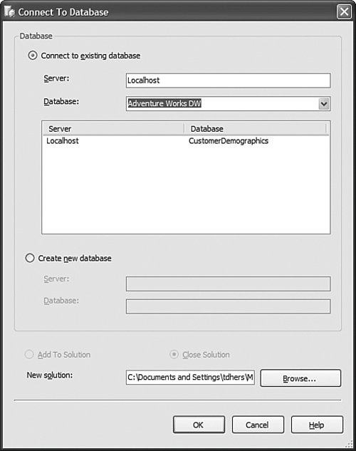 In the Connect To Database dialog, just enter the server name (and eventually instance name) and select the database to which you want to connect. Even though the object appears in the Solution Explorer, you are in live mode, not project mode. What does it mean to your experience? The designers and wizards will look the same, but saving means something extremely different. When working live against a database, saving means save changes and deploy changes immediately on the server. Some structurally breaking changes may result in forcing a reprocessing of the object. By contrast, in project mode, save just means save the changes in the XML file of this object; the live database is not impacted by this change until the project is redeployed. So when should you use project mode? In any other cases (different teams are developing and managing, or there are multiple developers), I recommend working in project mode. Working in project mode decouples the development cycle from the operational side. One can develop a new version of an application while users still continue querying the current version. Project mode also enables you to leverage a source control system to check in files, check out files, create multiple versions, and allow multiple developers to work on the same project simultaneously. Project mode also enables you to fully support the full life cycle of an application:
By default, projects are saved under the My Documents\Visual Studio 2005\Projects folder, but they can also be stored and retrieved from any file share as well (see Figure 13-18). Figure 13-18. Open Project dialog.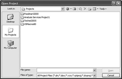 Because in project mode the object definition is saved in XML files in the project folder, do not forget to regularly back up this project folder if you are not using a source control system. How Do I Deploy a DB Across Servers?Well, in Analysis Services 2000, this was one of the top most-asked questions. Back then, the only answer was to use backup and restore to move the database over to a different server. It was a limited solution because Backup had a 2GB file size limitation and very often cubes were larger than this. With Analysis Services 2005, we do not provide one solution to this problem; we provide at least four: Deploy the project to a different server, copy the project file on a different machine, use the much revamped Backup/restore, or use the synchronization wizard. Let's review each of them. The first option is to simply deploy the current project to a different target server. This can easily be achieved by setting a different server name on the Project Properties dialog (see Figure 13-19). Figure 13-19. Project deployment options.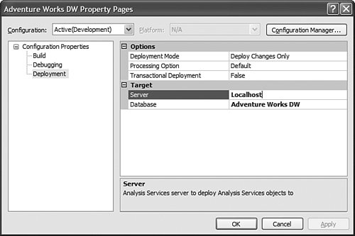 This is a very natural solution for moving from a development machine to a test environment or from a test environment to a production environment. Obviously this option is available to you only if you work in project mode as opposed to live mode against a server. The second option is to simply copy the project over to a different server and reopen it on that other server with the local BI development studio. Again, this project needs to be deployed on this new server to create the objects on the Analysis Server. Since the project is self contained, it is a very convenient option when you need to move a project between two servers that are on two different domains or that have no network connectivity between them. The third option is to use the much revamped backup and restore utility (see Figure 13-20). The Analysis Services backup and restore has become very similar to the SQL Server relational backup and restore feature. It no longer suffers from a 2GB file limitation. Unlike the two first options, this option enables you to not only move the database object's definition from one server to another but also to move the data as well. This is the preferred choice for moving data and metadata between two production servers. It is obviously the option to use to recover a database in case it becomes damaged. Figure 13-20. Restore Database dialog.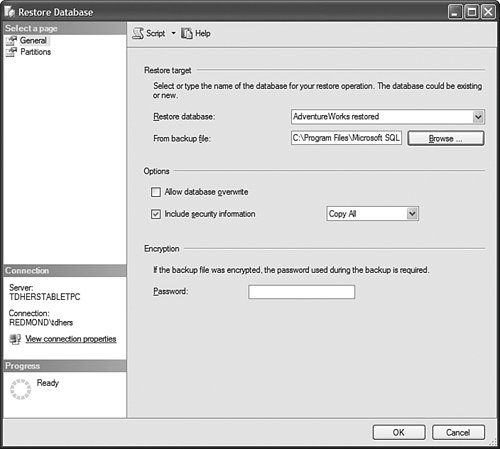 This solution provides greater flexibility in terms of moving data with or without security definitions. Indeed, you can select to overwrite role definition when restoring the backup file. You also have the capability to rename the database while restoring it. Finally, the fourth option is to use the synchronization wizard or command (see Figure 13-21). This functionality is very much similar to the replication capability of the relational database. It enables you to define a synchronization rule on a target server. That rule will automatically replicate the database from a source server to the server on which the rule is defined. Figure 13-21. Synchronize Database Wizard.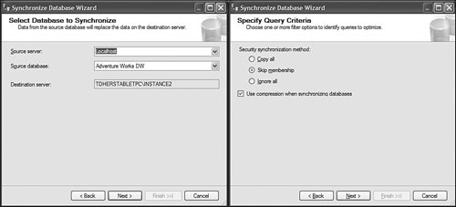 This functionality is particularly useful in a scale-out scenario. Indeed it might be very wise in such a situation, where a large number of concurrent users will be querying a fairly large cube, to decouple the server on which a database is processed from the server being queried by users. To do this, you may define an architecture with two servers: One server for processing the data, one for reporting against the data. In such an architecture you need to ensure at all times that both datasets are identical. You can use the synchronization wizard or command to periodically synchronize the data between the two servers. As with every command available through the SQL Management studio, a synchronization script can be generated. This option is actually offered during the last step of the wizard. A script example follows:
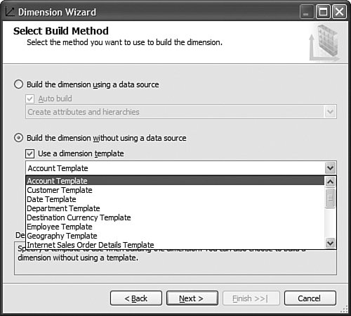
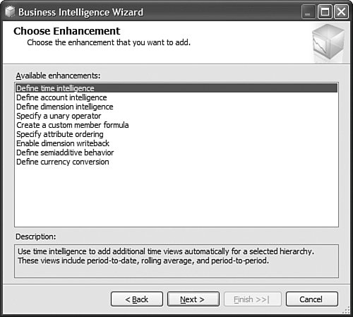
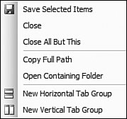
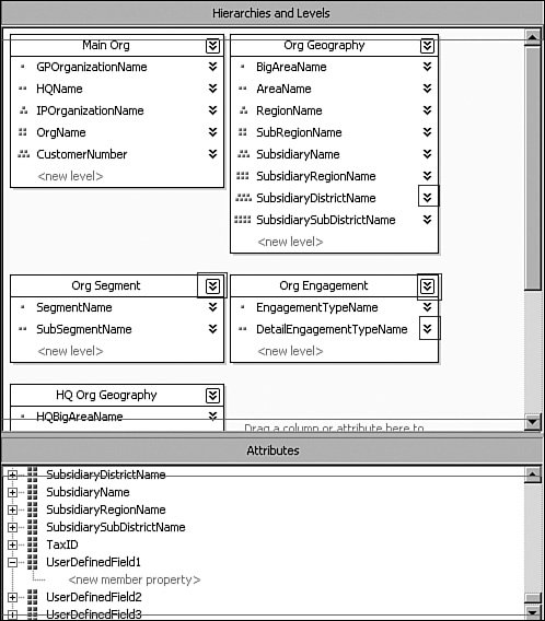
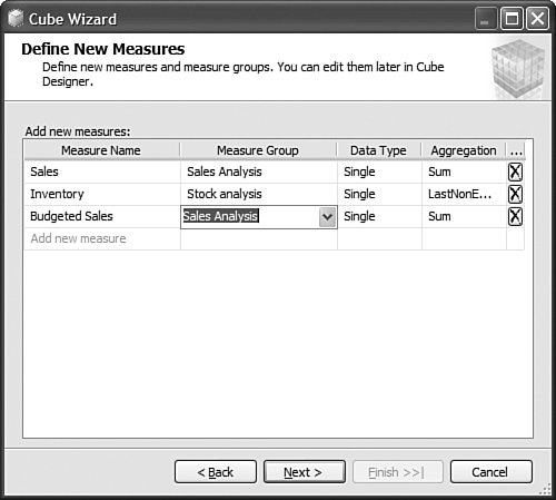
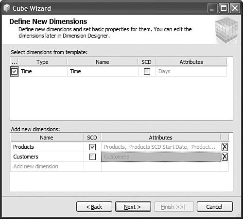
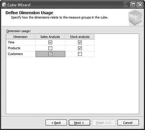
It is then fairly easy to schedule this synchronization to happen at regular intervals by using either SQL Agent jobs (see Figure 13-22) or Integration Services. Figure 13-22. Synchronization script automation through a SQL agent job.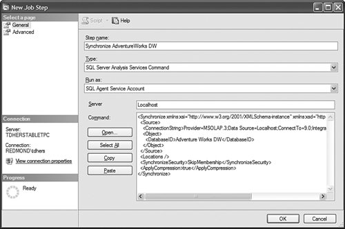 SQL Agent has been enhanced to now natively support two new types of steps: the SQL Server Analysis Services Command and the SQL Server Analysis Services query. In conclusion, you can see that Analysis Services has largely been enhanced in this area to provide you multiple ways to answer this question. Each option is better suited for specific business requirements and situations. How Do I Take an AS2K Cube and Enhance It with New AS2K5 Features?This scenario is very similar to the Migrate and Enhance option discussed earlier in this chapter. After an Analysis Services 2000 database has been migrated to Analysis Services 2005, you can enhance it by either importing it first into a project, or by connecting to the live database and starting to modify it to add translation, KPIs, or whatever else you need. The detailed procedure is described in the migration scenario earlier in this chapter. Just remember that migration migrates only metadata, and thus the database needs to be reprocessed before the data and metadata can be queried. How Do I Create New Templates for Cubes and Dimensions?One of the new ways to create a cube or dimension in Analysis Services 2005 is without using a preexisting data source. This is not necessarily one of the most advertised features, yet it is very useful for prototyping cube design before the underlying data becomes available. It is also an important feature when designing budgeting or forward-looking forecasting cubes for which data will only become available or be entered by users when the cube is put into production. Figure 13-23 shows an example of building dimensions with the Dimension Wizard. Figure 13-23. Building a dimension using a dimension template. When creating a cube or dimension without a data source, the database professional can decide to create the object from scratch or use a preexisting template. Out of the box, one cube template and nineteen dimension templates are provided. The templates are used to pre-fill measures, dimension hierarchies, and attributes while going through the wizard. These templates can be replaced and enhanced. Cube and dimension templates can contain a lot of pre-defined business content. As a result, it may be interesting to create many company templates so that when database administrators throughout the company create UDMs they do so using company-standard definitions. To replace or add a new template, simply use the XML file definition of the cube or dimension objects, as found in a project folder, and place it under the dimension or cube template folder under C:\Program Files\ Microsoft SQL Server\90\Tools\Templates\olap\1033 (see Figure 13-24). The path of the folder may be slightly different (that is, other than 1033) if the template needs to be made available in different locales. Here 1033 corresponds to the English U.S. locale. Figure 13-24. Selecting among the built-in dimension template XML files.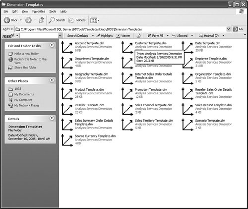 Why Should I Be Typing My Dimensions and Attributes with Dimension Types (Time, Currency, Account and so on) or Attribute Types?In Analysis Services 2000, dimension types (Regular, Product, Time, and so on) or level types (Year, Quarter, Month, and so on) already existed. Typing these objects was important mainly for the time intelligence of the cube. Indeed, for example, YTD and QTD MDX functions needed this information to behave properly and return results. Attribute types were also used by third-party vendors to add business intelligence and behavior based on the knowledge of the semantic meaning of the dimension or the level. For example, the Microsoft Mappoint OLAP Addin uses this information to determine which dimension and level contains the geographical data. Using this information, the Mappoint wizard pre-selects the correct dimension and level to use to map the data geographically. Figure 13-25 shows the Dimension Structure tab grid view used to view attribute types. Figure 13-25. Using the Dimension Structure tab grid view to view attribute types.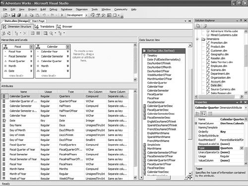 In Analysis Services 2005, dimension types and attribute types become even more important. The Analysis Services engine has been enhanced with more advanced logics and computations that depend on some semantic knowledge of the data. For example, the system is now aware of accounting logic based on knowledge of account type. (The ByAccount semi-additive aggregation computes aggregation based on the "Account type" type attribute.) The BI wizard can provide more or fewer options based on its detecting of a specific type of dimension (see Figure 13-26). For example, the currency conversion option needs to detect a currency type of dimension in the system to detect which measure groups are potentially the exchange rate measure groups. Figure 13-26. Business Intelligence Wizard available enhancements. How can you set dimension type or attribute type? Dimension type or attribute type can be set in many ways: through the Dimension wizard, cube wizard, BI Wizard, Cube Editor, Property pane, or the Dimension Structure Attribute pane of the Dimension editor (refer to Figure 13-25). Which attribute type does Analysis Services take advantage of? All the time-related attribute types or dimension types are still as important as in Analysis Services 2000. Currency types are now used by the BI wizard to detect exchange rate or source currency dimension. Account types are very important now for the ByAccount semi additive aggregation and currency conversion (for example, some account types are not to be converted.) Generally, my recommendation is that the more information you can give to the system and eventually a client application, the better. Even if some dimension types and attribute types are not used today by Analysis Services 2005 or a partner application, it doesn't mean that they won't be used in the future, either by a future version or service pack of Analysis Services or by third-party applications. If a type is not used it is simply ignored, so it cannot hurt to set them. Also, if you are building a custom application, you can query this information and thus take advantage of it to embed business logic and intelligence in your custom application, based on your knowledge of the semantic meaning of these objects. How Do I Make Visual Development Studio Look Like Analysis Manager 2000?It is actually fairly easy to customize the Visual Studio environment designers. Each pane can be moved individually. Figure 13-27 shows the standard BI Development Studio interface. Figure 13-27. BI Development studio before shell customization.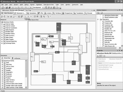 Simply move the Solution Explorer from the right side to the left side of the design environment (see Figure 13-28). Figure 13-28. Customizing the shell, using drag-and-drop operations on windows.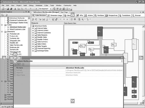 Similarly, just move the Property pane below the Solution Explorer in the left area. These changes are persisted across sessions. Now remember that even if you make the BI development studio look like Analysis Manager 2000, it doesn't necessarily mean that it behaves the same. Unless you are in live mode, the BI development studio is still working with only files, not live objects, as the Analysis Manager 2000 does. The other difference is that unlike Analysis Manager 2000, designers open as tab panes, whereas in Analysis Manager 2000, they open individually, one at a time, as modal dialogs. The benefit of non-modal dialogs is obvious, yet it requires more screen real estate. Tip Right-click on the tab area to split the designer screen in two to see two different designers side by side or one on top of the other (see Figure 13-29). Figure 13-29. BI development studio tab Context menu. Tip In Analysis Manager the property pane could be collapsed. In BI Development Studio, each pane can be pinned or unpinned. If unpinned, they collapse automatically when they lose focus. This is very convenient for maintaining as much usable screen real estate as possible (see Figure 13-30). Figure 13-30. BI Development Studio after customization.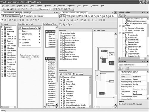 How Can I Produce Documentation for Every Object Contained in My Solution?Although AS2005 tools do not provide such built-in functionality, it is relatively easy to build a utility that can extract metadata and lay it out nicely on either an HTML page or a Word document. The key is to work in project mode, not live mode. If you work in project mode, then all the metadata is readily available in XML. Indeed, all objects are saved in Solution Explorer as XML files. A program that would be parsing these XML files and organizing the data in an HTML or Word document can be written in a few days or weeks by an intern. We are including a sample on the CD included in this book of such a documenter utility. This documenter utility works with relational databases, IS packages, and AS cubes and mining models (see Figure 13-31). As soon as the Documenter has been run and completes successfully against either server, it automatically generates an HTML-based document with the format shown in Figure 13-32. Figure 13-31. SQL Server 2005 Documenter.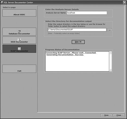 Figure 13-32. Documenter Summary document.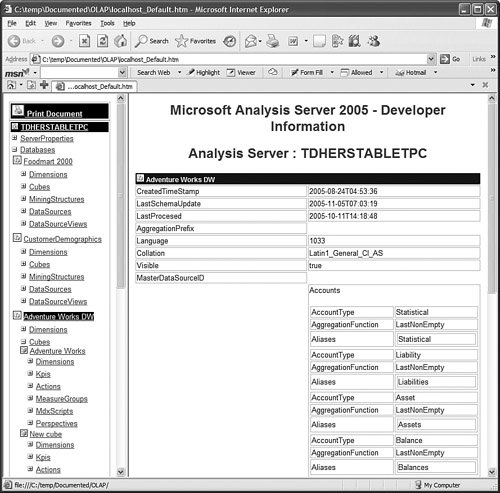 When Would Auto-scrolling During Drag-and-Drop Operations Help?Some databases are huge. Designing an OLAP solution on top of those databases can be a challenge. Taking into account that the most popular way of designing things in a UI is drag-and-drop operation, we added some auto-scrolling capabilities into UI elements. If your dimension has many attributes and those attributes are not always related to the key attribute of the dimension, then most probably you need to define attribute relationships (member properties) in the Hierarchies and Levels window or in the tree view of the Attributes window. If you drag an object understandable by the designer (columns from Data Source View or attributes or member properties) and hover the mouse cursor over the upper or lower borders of the windows for approximately one second, then the window scrolls its contents. If you hover the mouse cursor over a tree node in the tree view for about one second, then the node flips into its expanded state. The expanded node becomes collapsed while the collapsed node becomes expanded. The same thing happens with the Hierarchies and Levels window, but you need to place the mouse cursor at specific areas that you normally use to expand and collapse hierarchical objects with mouse clicks. Figure 13-33 shows the horizontal areas at the top and bottom that trigger auto-scrolling and, with the small square around the chevrons icon, the areas that trigger the change of the expanded state of the object associated with it. Figure 13-33. Attributes and hierarchies areas sensitive to auto-scrolling. The same thing happens in Data Source View. Some tables have many columns, and the shapes of the tables are sized smaller. The number of tables in the view can be high. When defining a relationship between two tables with a drag-and-drop operation, one can also benefit from auto-scrolling capabilities. The areas that trigger scrolling of the entire view and the areas that trigger auto-scrolling of the list views of the shapes representing tables are shown in Figure 13-34. Figure 13-34. DSV areas sensitive to auto-scrolling.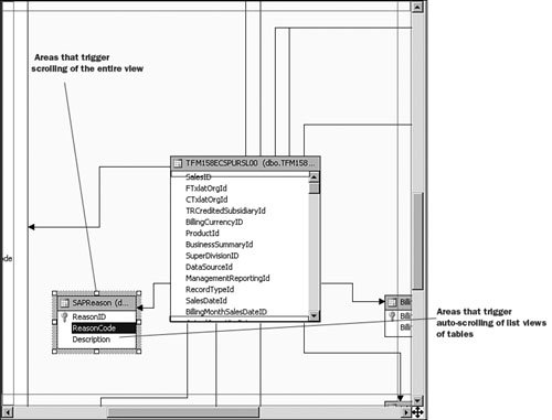 How Do I Use SQL in Cube, Dimension, and Partition Definitions?AS2000 had pieces of SQL spread around in the definition of cubes and dimensions. For example, the Source Table Filter might contain a WHERE clause and the Member Key Column properties might contain parts of the SELECT clause. Although this provided nice flexibility in defining the cube and dimensions, it had two drawbacks: 1) Cube and dimension definitions became dependent on the SQL dialect of the relational data source, and 2) SQL was spread out in separate pieces that were difficult to locate and validate because each piece was only a part of the SQL eventually used by the server. In AS2005 we've consolidated the SQL into the Data Source View object (DSV). To do the equivalent of setting the Source Table Filter in AS2005, right-click on the top of the table in the DSV that you want to filter and choose the Replace Table > With New Named Query context menu. Then simply add your own WHERE clause to the query to be used in place of the direct reference to the table. (Use Ctr-Enter to add new lines to the query.) When you are finished, the named query has replaced the table (it has the same ID) and your cubes and dimensions that previously referred to the table in the DSV now refer to the named query. To do the equivalent of setting the filter on a partition in AS2005, you can use this same technique of replacing the DSV table with a named query. Note that partitions can be defined to point to a table in a DSV or directly to a table in the data source, and only those partitions that point to the table in the DSV will be affected by replacement of the DSV table. When you have multiple partitions, you will want each partition to have a different filter. To do this, you can change the source of the partition to be a query containing the appropriate WHERE clause. You can also change the source to be a different table, named query, or view with the same structure. To do the equivalent of putting SQL in the Member Key Column or Member Name Column, you can replace the table in the DSV with a named query as already described or you can create a new named calculation, also available by right-clicking on the top of the table in the DSV. Named calculations provide a way to define additional columns on a table based on SQL expressions. Named calculations are available only on tables, but if you want to add a column to a named query, simply edit that named query. How Can I Prototype a Cube Rapidly Without Prerequiring Any Existing Data Sources?This is one of the very powerful yet most unknown features of the new release. Unlike in the previous release, a cube or a dimension can now be built without requiring a previously built underlying data source. Let's look at the Cube Wizard, for example: The second option in the Select Build Method page enables the user to custom-build a dimension with or without the help of a template. Dimension and cube templates are discussed in a previous section. The user is consecutively presented with the option to create new measures (see Figure 13-35) and new dimensions (see Figure 13-36). Then he can associate the dimension with measures and give a name to the cube (see Figure 13-37). Figure 13-35. Define New Measures. Figure 13-36. Define New Dimensions. Figure 13-37. Define Dimension Usage. After this wizard is completed, you can continue editing dimensions and cube objects in each designer by adding or removing measures, attributes, or hierarchies (see Figure 13-38). Figure 13-38. Using the link in the Dimension Structure tab DSV pane to generate the Data Source View.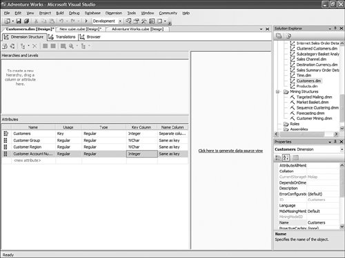 You will eventually need to use the Schema generation wizard to generate the underlying tables to store this information (see Figure 13-39). Figure 13-39. Dimension structure pane after the Data Source View has been generated.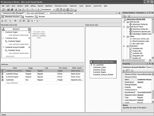 After you have completed this simple step, then it becomes just a matter of using the dimension Writeback capability (assuming the Writeback property was set to True; it is False by default) to start entering dimension members and populating each dimension (see Figure 13-40). Figure 13-40. Populating dimension members, using Dimension Writeback.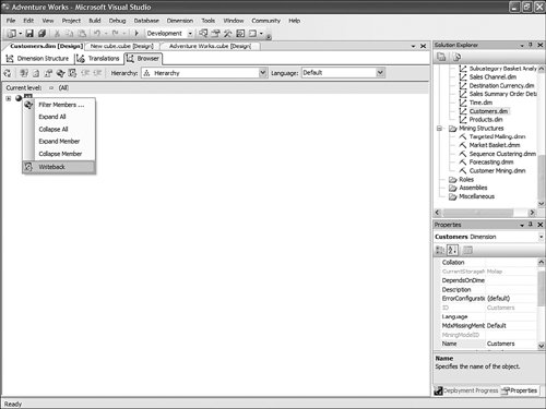 In a few minutes, a cube is created with dimensions populated with members (see Figure 13-41). Now using any Excel add-in or partner or customer application, data can be rapidly entered to populate the cube itself. Figure 13-41. Newly created dimension members, using Dimension Writeback.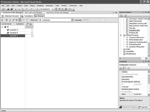 How Can I Easily Use Test Data to Speed Development of Cubes and Dimensions?Often when designing a cube or dimension, you'd like to design and test the structure and calculations on a smaller set of data than what you will deploy on. This is particularly useful in designing calculations, in that it allows you to deploy more quickly and test calculations on known data with which you can more easily verify your results. This section was written as a tips and trick section by our AS Tools Development lead, Matt Carroll. Using Replace TableA simple way to do this when just a few tables are involved is to use the Replace Table feature of the DSV:
For newly created cubes, the default partition of a measure group whose table has been replaced automatically references the new table or named query. For old cubes or a cube on which you have modified the partitions, be sure to check each partition. Partitions that reference DSV table objects automatically refer to the new table or named query, whereas those that reference DS table objects or queries will not be updated. (It is generally recommended that you design partitions after you've completed the design of cube and dimension structure and calculations.) When you are finished testing and wish to return to using your production data, simply repeat the preceding steps and replace the table with the original table containing your full data set. Modifying the Data SourceSometimes when many related tables are involved, it's easier to have a separate test relational database. If you have a separate test relational database, then you can very easily use this database by editing the connection string in the Data Source object used by your cubes and dimensions. When you want to return to the production data, just edit the connection string of the Data Source object again. If the project is shared with other people, has multiple data sources, has other configurable properties such as a target server or database that you'd like to control, or if you just can't seem to remember your connection strings, you may want to follow the more formal process of defining multiple project configurations. The connection string property of the Data Source object is a configurable property, and its value is stored in the active configuration. This enables you to easily switch connection strings by simply switching active configurations. To create a new configuration, follow these steps:
To switch active configurations, follow these steps:
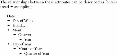
To set the connection string of a data source associated with the active configuration, simply edit the data source normally and the connection string will automatically be saved as part of the active configuration. Another alternative is to create a new Data Source object and change the Data Source View to temporarily point to this new Data Source object. This tends to be more complicated because it involves more steps, partitions which directly refer to the Data Source will not be updated, and it cannot be maintained through configurations. How Do I View Sample Measures Data in the Cube Wizard?When using the Cube Wizard, measures and measure groups can be generated automatically. The problem is that without seeing the actual data, it is sometimes very hard to make a decision concerning which measures should be used. The solution is simple: Just right-click on any measure and a new window with sample data appears. How Do I Compare Two Measure Groups' Dimensionality?One of the major enhancements of the UDM is the capability to model data from different data sources, at different levels of granularity, and in different dimensionality within the same cube. Potentially an entire data warehouse or even multiple OLTP databases and LOB applications can be modeled within the same cube. As a result it is very likely that you can find yourself building a cube with well over a dozen measure groups and dimensions. In this case, it can become hard to compare the dimensionality of two measure groups or to do an analysis that would yield the measure group in which a specific dimension would participate. The Cube Designer offers a specific dimension usage tab for this reason (see Figure 13-42). Figure 13-42. Dimension Usage tab, unfiltered.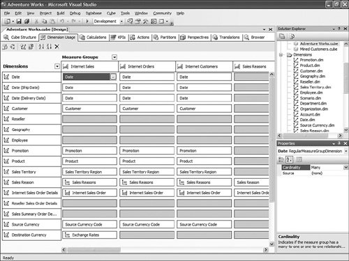 This tab is great because it offers a grid view of the dimensions and measure group relationships. Yet the span of this grid can sometimes greatly exceed the size of the users' screens. For this reason, this designer offers the possibility to filter one or multiple measure groups in columns and/or one of multiple dimensions in rows. This is particularly useful if you need to compare two specific measure groups' dimensionality. By just selecting these two measure groups you have now reduced the view to only the dimensionality of these two objects (see Figure 13-43). Figure 13-43. Dimension Usage tab, filtered by Measure groups.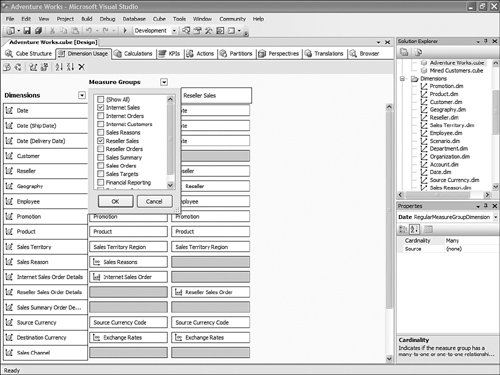 Similarly, if you rapidly need to find in which measure group a dimension participates, just filter on this dimension in rows and you can identify the measure groups that use those dimensions. Again using the measure group filter, you can now reduce your view to only these measure groups where this dimension comes into play (see Figure 13-44). Figure 13-44. Dimension Usage tab filtered by dimensions.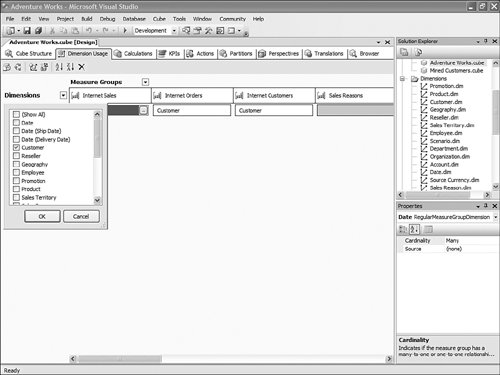 Tip The value shown in the cell of each intersection in this grid represents the granularity, which means the level of the dimension, at which the measure group intersects. How Can I Have a Measure Group with a Level of Granularity Above the Key?The Dimension Usage tab of the Cube Designer enables you to view and edit the relationships between a specific measure group and dimensions. At the intersection of rows and columns, the cell represents the granularity at which a measure group in column is dimensioned by the dimension in row. The granularity represents the attribute that is the lowest level of granularity of the data for this dimension found in the measure group. Often the granularity of the dimension is also the granularity of the measure groups. But sometime the measure group data is not as granular as the dimension. For example, if a cube contains a Product dimension whose lowest granularity is the SKU level, it is very likely that the actual sales are reported at the SKU level, yet when it comes to Budget or forecast data, this is another story. Budget data is most often entered during the planning cycle at a higher level, such as Product group or Product category. As a result, Analysis Services enables setting the granularity of a specific measure group at a higher level than the dimension key level. This can be achieved by simply clicking on the cell that represents the intersection between a measure group and dimension. This brings up the Define Relationship dialog (see Figure 13-45). Through this dialog the bindings between the dimension and a measure group can be set to a different level of granularity. Figure 13-45. Define Relationship dialog.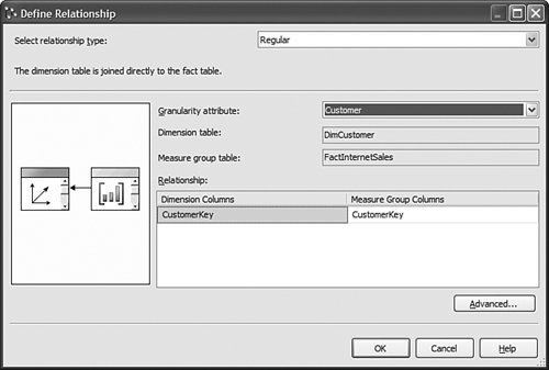 At first look this seems pretty easy, but the new attribute-based architecture makes some of the mechanics of handling this in the engine slightly more complex. The following sections written by Matt Carroll explain the importance of key uniqueness and attribute relationship when setting a measure group granularity above the dimension key. As in AS2000, AS2005 enables you to have a measure group joined to a dimension above the lowest level of detail in that dimension. This is common with the time dimension if, for example, your sales are recorded daily but your inventory levels are recorded monthly. For this to work, the server must know what levels of detail are above the selected granularity and thus are still available for slicing the measure group. In AS2000 this was easy because a dimension contained only a single hierarchy and there was no notion of attributes, but only levels within this single hierarchy. In AS2005, dimensions are more flexible and contain many attributes. Each attribute may be contained in zero, one, or many user-defined hierarchies. This flexibility means hierarchies alone do not usually provide sufficient information to the server to know which attributes still apply to the measure group. Relationships Between AttributesAS2005 introduces the idea of relationships between attributes to solve this problem (as well as to define member properties). By definition, all attributes are related to the key attribute, so if you know the value of the key, you know the value of any attribute. However, if you use a non-key attribute for the granularity of a measure group, the server must know what attributes are related to the granularity attribute and thus can be used to slice the measure group. To make this work you may need to define additional relationships between attributes. In the dimension, these relationships are defined by AttributeRelationships (called MemberProperties in earlier beta 1 and 2) and can be seen by switching to the tree view layout (now the default) of the attribute list. Let's look at an example. Given a time dimension with the following attributes
Given all this, if you select the key attribute (Date) as the granularity attribute, all attributes in the dimension apply to the measure group because the key attribute directly or indirectly implies the values of all attributes in the dimension. If you select Day of Week as the granularity attribute, then only Day of Week applies to the measure group because it implies no other attributes. If you select Month, then the attributes Month, Quarter, and Year apply to the measure group. Notice that if you select Month of Year as the granularity attribute, Quarter of Year applies to the measure group, but Year does not because the Quarter of Year (e.g., Q1) does not imply any year. Making the distinction between Month and Month of Year is important in AS2005 and is easily overlooked. Importance of Key UniquenessIn AS2000, a month lived in a hierarchy, so its meaning was determined by the hierarchy. So if the hierarchy contained Year-Month, then there was no confusion that it was Month (Q1 2000 - year specific) and not Month of Year (Q1 - year neutral). In AS2000 if the column of month contained just Q1, but it was used in a hierarchy with a year, then you would set UniqueKeys=False to tell the system to combine the key column of that level with the key of the level above to get unique key values. In AS2005, each attribute lives independent of hierarchies, so you must define its key as using both the month and year columns in the attributes key columns collection. How Do I Change Calculation, Action, or KPI MDX Templates?One possibly not very well-known enhancement in Analysis Services 2005 is the open extensible template architecture. Calculation templates are very useful to jump-start defining new business logics. The Calculation template, KPI template and Action Templates tab contain well over 100 definitions of the most popular business logics, from how to calculate growth, YTD, and moving average, to more financial ones such as EVA (economic value added), DSO (days of sales outstanding), or return on asset formulas. But often a consulting company or even an IT department may look at customizing this list to a specific business domain or to the specific taxonomy of a company. All these templates are defined in a clear XML document. This XML template document can be found under C:\Program Files\Microsoft SQL Server\90\Tools\Templates\olap\1033. The 1033 represents the locale identifier (U.S. English here) under which these templates are stored. This also means that this template can be localized and found in different sub folders. The template filename is MDXTemplates.XML. The structure of a template is pretty straightforward. For example, a typical Year to Date MDX calculation will be described as follows:
An action template will look like this:
And a KPI template is defined as follows:
Obviously, different types of templates have different tags, but these tags map to the properties of each object generated (calculated member, action, KPI, named set). Each MDX expression used in these templates is tokenized, using the following convention: <<Token name>>. This convention is not required and is just here for practical purposes. As many templates can be added or removed as needed. After the file is edited, it just needs to be placed in the same folder with the same name, and the change will be picked up by Development Studio next time it is started. Should I Use the KPI Display Folder or KPI Parent Property?Beyond Goal, Trend, or Status a, Key Performance Indicator (KPI) has two properties that enable that KPI to be categorized. The first one is the KPI display Folder. This property is very useful for categorizing a KPI under one or more strategic goals. These strategic goals can themselves be categorized under one or more business perspective. The KPI can belong to one of multiple display folders. Display folders can be nested with no limit of nesting. As a result, a KPI display folder can be defined as KPI Display Folder = Folder1\SubFolder1\...; Folder2\SubFolder2\...;... Display folders are simple categorization mechanisms. Display folders do not have Goal, Trend, or Status values. In contrast, it is sometimes important to show KPIs in a hierarchical manner. In this case, the parent KPI property shall be used. This property makes it possible to define a hierarchy of KPIs. When a KPI is set as a parent of another KPI, the other KPI is automatically displayed beneath the parent KPI. The display folder of the children KPIs is then ignored. Figure 13-46 shows a parent KPI being defined in the KPIs tab. Figure 13-46. Defining the Parent KPI using the KPI tab.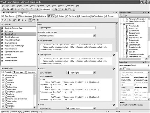 So the question arises, when should one be used versus the other? Well, if the categorization is needed to model a business or scorecard type of organization, then the display folder is the one to use. But if the KPIs themselves need to be displayed in a hierarchical manner, then the parent KPI property should be used. Figure 13-47 shows an example of using both the display folder and parent KPI properties approaches. Figure 13-47. Using both Display Folder and Parent KPI properties.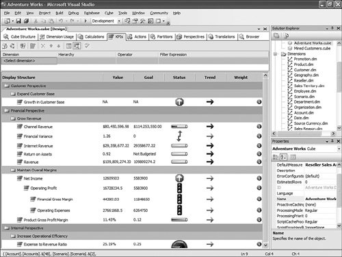 But categorization and hierarchy are often not enough. Most companies that follow a balanced or business scorecard methodology also often like to have some sort of master indicator that would give the overall health index of the entire corporation. Building this Company Health Index is not very difficult. The Company Health Index is itself a KPI, the values of which depend on other KPIs. But not every KPI is equally important as others for the company. Depending on the overall company strategy, some KPIs may be more critical to the overall Health Index of the company than others. This is where the KPI weight property comes into play. Each KPI must be assigned a weight. This way its importance or criticality can be taken into account when computing the overall Company Health Index. Let's look at how such a computation would be set up. Assume 5 KPIs with the following associated weights: KPI1 (1), KPI2 (1), KPI3 (2), KPI4 (2), KPI5 (1). You can now build the Overall Company Health Index (OCHI). Its value should be the aggregation of the status of all the KPIs, weighted by their respective weights: OCHI Value = (KPISTATUS(KPI1) * KPIWEIGHT(KPI1) + KPISTATUS(KPI2) * KPIWEIGHT(KPI2) + KPISTATUS(KPI3) * KPIWEIGHT(KPI3) + KPISTATUS(KPI4) * KPIWEIGHT(KPI4) + KPISTATUS(KPI5) * KPIWEIGHT(KPI5) ) / (KPIWEIGHT(KPI1) + KPIWEIGHT(KPI2) + KPIWEIGHT(KPI3) + KPIWEIGHT(KPI4) + KPIWEIGHT(KPI5)) The OCHI goal is obviously 1. The OCHI status can be set to any expression that suits your company's objectives. It is as simple as this, and it provides great value to business users and executive decisionmakers. Because the OCHI KPI is a KPI like any others, it can very easily be queried and retrieved, using any client tool supporting MDX. The KPIVALUE(), KPIGOAL(), KPITREND(), and KPISTATUS() MDX functions can be used against this OCHI KPI. Thus Reporting Services, Microsoft Excel, as well as partner tools such as Proclarity or Panorama can expose this OCHI KPI. To see more examples of how to query and embed KPIs in your custom application, please look at the three samples provided in the appendices:
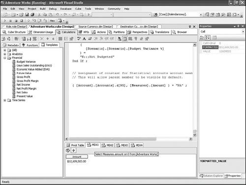
How Can I Rebuild My Own KPI Browser, Similar to the One Available in BI Development Studio, and Embed It in My Application?Often, when presenting the product, people ask us whether we are making the KPI debugger/browser available as a control. We currently are not, but on the book's CD you will find a sample that will show you how to build a very simple ASP.NET application that rebuilds a similar control. This sample was built in a week by a French Microsoft consultant, Olivier Pieri, for one of his customers. KPIs are accessible through MDX functions (KPIVALUE, KPIGOAL, KPITREND, KPISTATUS, KPIWEIGHT, and so on), so they can be queried like any other measures in the cube. So like any application that would attempt to embed analytical capabilities using MDX, the very same approach can be used with ADOMD.NET to query and display KPIs. The KPIViewer sample enables the user to connect to a server, select a database, and then be presented with the list of available KPIs (see Figure 13-48). Figure 13-48. KPI Viewer Connection page.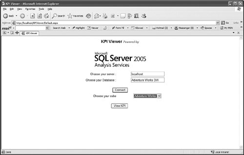 By default all KPIs are displayed for the default member (most likely all members) of every attribute of every dimension (see Figure 13-49). Figure 13-49. Default list of KPIs, unfiltered by any dimensions.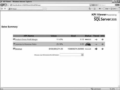 A control at the bottom enables the user to select a dimension and a hierarchy or attribute on which to drill down when clicking on a specific KPI. It is possible to select multiple attributes coming from the same or different dimensions successively to drill down in a specific KPI. The path for the dimensions/attributes combination is displayed at the top of the KPI list (see Figure 13-50). Figure 13-50. KPI list, filtered on time dimensions.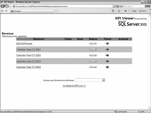 The sample can be found on the CD-ROM. The sample folder contains installation instructions, as well as all the source code and images needed. How Do I Use the Cube Debugger as a Calculation Builder?The new SQL Server BI development studio offers a unique capability in the BI Market: a full-blown MDX debugger. This is one of the side benefits of integrating with the Visual Studio development environment. Some of the native Visual Studio debugging services enabled us to build such a capability into our designers. The following section has been written by one of our most talented developers, Andrew Garbuzov, who actually coded the MDX debugger support in our Cube designer. Many users tend to build certain complex calculations and immediately try to verify the correctness of the step they have just completed. This is especially true if the cost of verifying the calculation correctness is not too high. In the Business Intelligence Development Studio, users can build cube calculation scripts on the Calculations page of the cube builder. They have the option to edit the script directly or create calculations one at a time in the user interface windows. Those who prefer creating the script in the text editor rather than in the UI might find the debugger to be a calculations script building tool created just for them. It is often true that a database designer might want to create the database to be successfully deployed without any calculations, and after that design and apply the calculation script. After you successfully deploy the database you can debug the cube. All you need is to invoke the Debug, Start menu command on the Calculations page of the cube builder. The debugger will run and stop at the first statement. The idea is that you would type your statements, execute them, and explore the cube's state in the pivot table or MDX watch windows. If you do not like the results, you modify your script. Tips for Creating CalculationsTo help you create good calculations, we have included the following tips:
Tip To make it easier to debug a specific calculation, it is often recommended to break down a calculation into as many calculations as possible. For example, imagine that a calculation is made of three sub components: A = (B/C + D/E) / F. It becomes much easier to debug and find out which portion of the calculation may not be behaving properly if you write the calculation like this instead: A1 = B/C A2 = D/E A = A1 + A2 A = A / F A1 and A2 enable you to debug each numerator component independently. This saves you a lot of time trying to isolate an issue, if one were to arise. Because the AS engine now handles recursions natively, the last two statements are perfectly valid. The second A= statement reads the value of A on the right side of the equal sign from its previous statement and applies it to the new iteration. After your calculations return the expected result, the four calculations can be merged into one again. How Do I Automate Loading Translation Strings into My Project?This is actually a fairly simple process. But first let's review what translations are. Cubes, dimensions, and mining models all contain metadata. This metadata is made up of descriptions, captions, property names, and values (see Figure 13-53). For dimensions, in addition to metadata, dimension members' names can also be translated. Loading dimension member name translation is just a matter of creating an extra column in the relational table where these members are defined. On the other hand, the metadata is persisted in the XML files describing each of the objects. Obviously this applies only to the case where you work in Project mode and not in Live mode. Figure 13-53. Cube Designer Translations tab.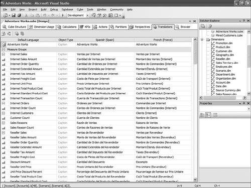 So the key here is that these translations are persisted in the XML file. This XML file can be edited outside of the designers. You can view the XML file in XML view by simply right-clicking on the cube or dimension name in the Solution Explorer and selecting the View Code menu item (see Figure 13-54). Figure 13-54. Solution Explorer context menu. Now all that needs to be done is to isolate the translation block for each piece of metadata: <Translations> <Translation dwd:design-time-name="translation1"> <Language>3082</Language> <Caption>Adventure Works</Caption> </Translation> <Translation dwd:design-time-name="translation36"> <Language>1036</Language> <Caption>Adventure Works</Caption> </Translation> </Translations> This example shows the translation block for the database name. The Language tag represents the LCID (ID of the Locale) of a specific language. As many can be created and added as languages that need to be supported. A little utility can rapidly be built to parse these XML files and extract the metadata field in an Excel spreadsheet, for example. Such a spreadsheet can then be sent to various members of the corporation to fill up the translations for each metadata field. After these translated fields have been completed, a similar utility can read them from the spreadsheet and place them in the appropriate translation block in the XML document. Saving the XML document and then redeploying it to the server will be sufficient to make these translations become available on the production server. How Do I Automatically Create Partitions for a New Data Set?One of the typical data warehouse challenge is refreshing the various parts of the data warehouse after the OLTP or LOB application has received new transactions. But the data warehouse is often made of several components: the relational data warehouse as well as the dimensional UDM or data marts. One of the issues is then to ensure that the UDM data marts are updated as simultaneously and transparently as the relational data warehouse component itself. There are several aspects to updating a UDM based on updates in the data warehouse. Often in a well structured data warehouse, a table partitioning strategy will have been defined to handle and organize new daily, weekly, monthly data. If such is the case, then one of the first challenges is to create the corresponding OLAP partition for each table partition. In the AdventureWorksDW set of samples, Dave Wickert from the SQL BI Systems team has created such a sample. It can be found in the following location: C:\Program Files\Microsoft SQL Server\90\Samples\Integration Services\Package Samples\SyncAdvWorksPartitions Sample\SynAdvWorksPartitions. After the OLAP partitions are automatically created for every new table partition, it is important to ensure that the data remains up to date with the relational data warehouse when it is updated. For this I recommend setting all the newly created partitions in proactive cache mode. Proactive cache is a great and easy way to let the cube partitions refresh themselves when new data is loaded in the relational partition. The recommended mode is Automatic MOLAP, but advanced settings enable you to customize the latency and refresh the frequency with which the cache is updated (see Figure 13-55). Figure 13-55. Setting partition storage to Automatic MOLAP (proactive caching).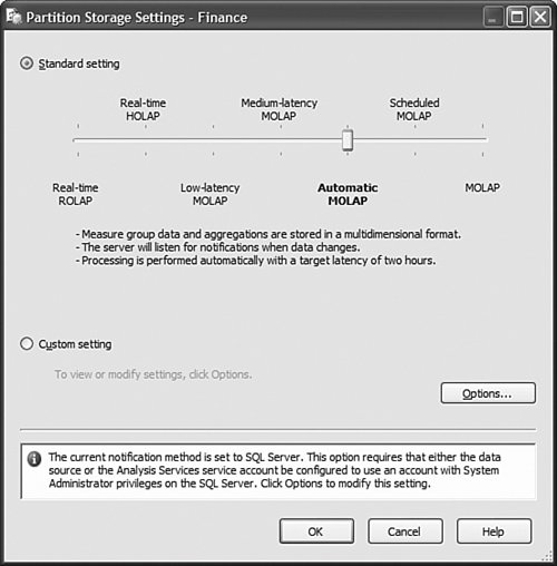 What Is the Difference Between the Cubes Filter Component and the OWC Filter in the Cube Browser Page?As discussed in the KPI section, the filter control generates a subcube (one for each row in the filter control), whereas OWC filters generate a more traditional WHERE clause. The main advantage I see of the Filter component is the capability to progressively restrict the cube space as you define successive filters. This is particularly useful when creating reports that use attributes with many members. It also enables much more sophisticated filtering. For the AS2000 user or the beginning user, using the OWC filter clause is more intuitive and simple. Figure 13-56 shows the Cube Browser filter components and Embedded OWC filter area. Figure 13-56. Cube Browser filter components and Embeded OWC filter area.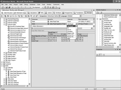 How Do I Test My Roles and Security?In AS2000, testing role security was done from the Role Manager dialog. Because now an AS database can be either created or edited in Live or Project mode, we had to slightly modify this behavior. Indeed, to test security you have to be able to access the live server, which is not necessarily feasible when working in project mode. Thus the AS development team decided to change the approach we had in AS2000. So with AS 2005, the testing role can be achieved directly through the cube browser that can be found in SQL Development Studio or BI Development Studio. When starting the Cube browser, the second icon that can be found on the toolbar allows the Database Professional to change the context under which the cube should be browsed (see Figure 13-57). Figure 13-57. Testing Dimension security by changing Role or User context.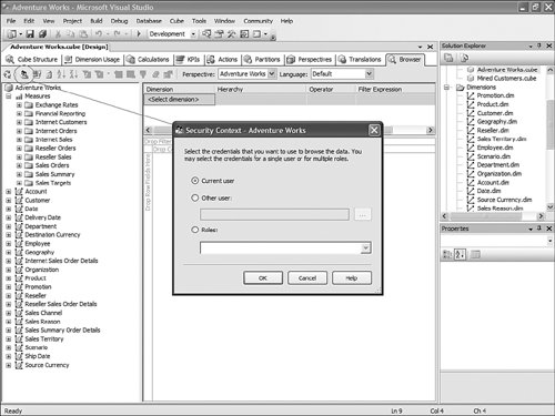 To change the context, you can choose to switch the current user with a specific selected username or one or multiple roles. This mechanism enables the database professional to test both cell security as well as dimension security. How Do I Change Time Intelligence Templates?The Time Intelligence path of the BI Wizard is a very valuable tool because it offers a very easy way to add most of the more common time-based business logic to your cube. Things like Year-to-Date, Year-over-Year growth, and 12-Month Moving Average can be added in the cube in a matter of literally three clicks (see Figure 13-58). Figure 13-58. Choose Additional Time dimension calculations. But often a consulting company or even an IT department may look at customizing this list of predefined time-based business logic to a specific business domain or to the specific taxonomy of a company. All these templates are defined in a clear XML document. This XML template document can be found under C:\Program Files\Microsoft SQL Server\90\Tools\Templates\olap\1033. 1033 represents the locale identifier (U.S. English here) under which these templates are stored. This also means that this template could be localized and found in different sub folders. The Template file name is TimeIntelligence.XML. The structure of a template is pretty straightforward. For example, the 12-Month Moving Average calculation will be described as follows
The RequiredLevelGroups element is defined when the time-based business logic is presented to the user. Indeed, not every time-based business logic makes sense for every time dimension. For example, if a dimension doesn't contain a Quarter level, then all business logic related to Quarter (for example, Quarter to Date, Quarter over Quarter Growth) is not presented to the users. These level types should map to the Time Attribute Type list. And the business logic is displayed to only the user of the selected hierarchy containing levels, based on which attribute type property has been set to one of these attribute types. The token used in the formula section cannot be any token (unlike for MDX and KPI templates). The same token must be used in a custom-built formula. Not all of them may be needed, but if the custom logic needs to reference the selected dimension, hierarchy, or level, then these exact token must be used. The BI wizard replaces these tokens at runtime with the matching value from the cube. As many time templates can be added or removed as needed from this file. After the file is edited, it just needs to be placed in the same folder with the same name, and the change is picked up by the Development Studio next time it is started. How Do I Document Changes Generated by the BI Wizard?The BI Wizard can turn just one Boolean property from true of false, or it can change dozens of properties and create huge MDX scripts. If you want to document all those changes, simply, click on the tree view while on the last page of the wizard, and press Ctrl+C. This puts the whole tree view into the clipboard in a format that can be nicely pasted into Excel, Word, or even Notepad. How Do I Bring Pictures into My UDM?The UDM supports pictures natively. If installed, you can open the AdventureWorksDW AS Database project that can be found under: C:\Program Files\Microsoft SQL Server\90\Tools\Samples\. Two versions of the samples are installed for the Enterprise SKU, and one is installed for the Standard SKU. Open one of the versions of SQL Server that is installed on your server. When the project is open, edit the Product dimension, select the Large Photo attribute, and edit its properties as shown in Figure 13-59. Figure 13-59. Set the MimeType property for the Large Photo attribute in Dimension Designer.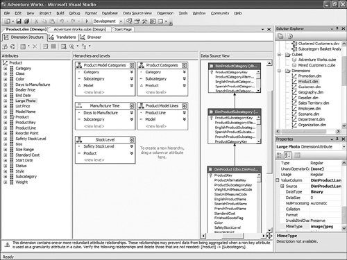 The ValueColumn set of properties determines the Image column to which the attribute is bound. In addition, it is important to set the DataType to Binary; this is so the UDM knows it is a picture. Then, and this is not set in the sample project by default, for this image to be rendered in Reporting Services and Report Builder, you need to set the MimeType to the type of the image stored in the relational database. In the case of the Product Large Photo, the type is Jpeg, so the MimeType value must be set to Image/Jpeg. After this change is done, the project must be redeployed, and if the Report Builder model was already generated, it must be regenerated. As soon as this is done, you can use Reporting Services Designer or Report builder to build a nice-looking report, entirely built on top of the UDM, that would not just display the entity's attribute, metrics, and KPIs, but pictures as well (see Figure 13-60 and Figure 13-61). Figure 13-60. Report builder Report design phase.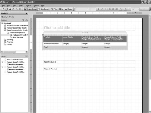 Figure 13-61. Report builder report preview.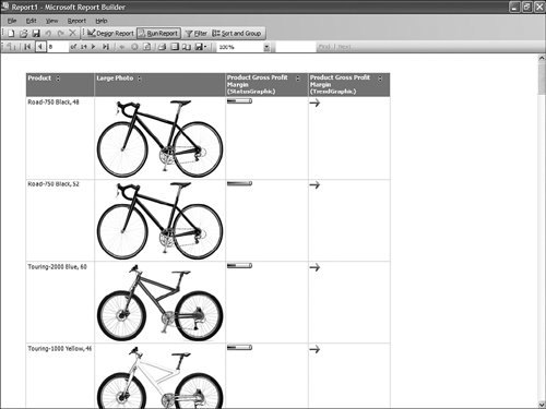 Which Tree Views in the User Interface That Support Multiple Selections Might Help in My Case?In many areas of the designer, multi-object selection is available. This is often very practical because the Visual Studio shell, for example, enables a common property to be edited for all the selected objects (as long as they all support the same property). In the Dimension designers, for example, the Tree View supports an alternate grid view, as shown in Figure 13-62. Figure 13-62. Dimension Designer Builder, tree view.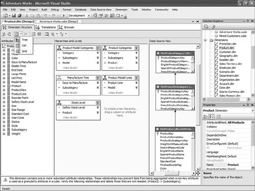 After the view is switched to grid (see Figure 13-63), then multiple attributes can be selected. All their common properties are displayed in the property pane and can be set for all the attributes at once. Figure 13-63. Dimension Designer Builder, grid view.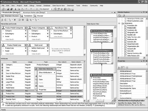 In addition, the context menu makes it possible to create a hierarchy out of these attributes in one click. In similar ways, many areas of the Cube, Mining Model, or Security designer enable you to select multiple objects in a tree or grid view. When in a grid view, you can edit a column for all selected objects by simply using the F2 key. How Do I Set Up a Dimension with Multiple Parents Rollup with Weights?Here is a situation where a member needs to be modeled so that it rolls up to multiple parents with different weights. This is perfectly feasible in AS2000 and AS2005 if you use the following steps. First let's take care of the member-to-multiple-parent issue:
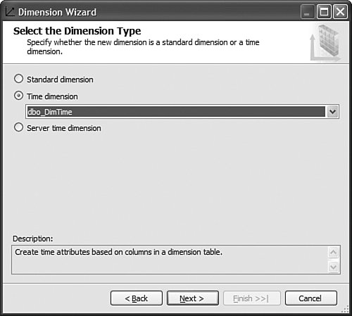
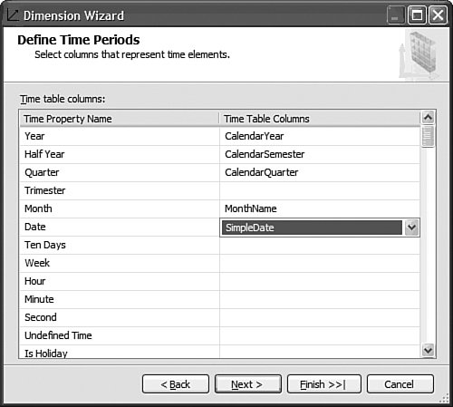
Now let's add a weight and/or unary operator to these members to control how they roll up:
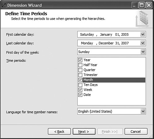
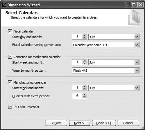
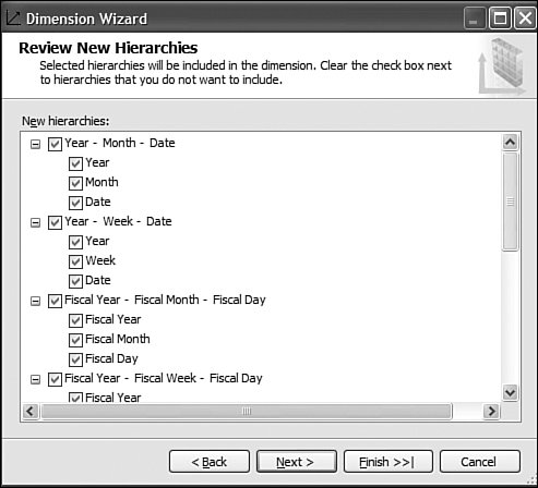
This is pretty straightforward to set up through the tool, but this question has been asked very frequently in the newsgroups, so we felt it would be appropriate to give the answer in this book as well. How Should I Build the Time Dimension?When building a time dimension, multiple options are available in the Dimension Wizard, as shown in Figure 13-64. Figure 13-64. Dimension WizardTime Dimension. So which option should be used? Well, it depends on whether your data source already contains a time table or not. If the data source contains a table where the time frequency and periodicity is defined, then the database professional should use the time dimension option. In the following steps, the wizard (see Figure 13-65) then enables the user to map the column of the table with a dimension attribute type (Year, Month, Day, etc.). Figure 13-65. Dimension Wizardtime periods definition. This step is very important because it makes it possible to assign an Attribute type with each of the dimension attributes. In addition, the wizard generates the appropriate hierarchies automatically. The second option is the one to use if no time table is available in the data source. In this case, the wizard builds a server-based time dimension. The wizard then lets you create the dimension by hand while providing a lot of advanced business calendar options (see Figures 13-66 through 13-68). Figure 13-66. Dimension Wizard Calendars Definition: Time Periods. Figure 13-67. Dimension Wizard Calendars Definition: Calendars. Figure 13-68. Dimension Wizard Calendars Definition: Reviewing Hierarchies. This path of the wizard automatically generates the hierarchies based on the options chosen. As you can see in Figures 13-6613-68, the five most common business calendars can be set up at once through the wizard. The hierarchies are generated with the dimension key being a time stamp. As long as the fact data also have a time stamp, this new dimension can then be linked to any fact data. How Do I Execute Multiple MDX Queries from SQL Server Management Studio?If you want to execute multiple queries against cubes within the database, then you can do so within SQL Server Management Studio. This section was written as a Tip and Trick by Andrew Garbuzov, who developed all the MDX, DMX, and XML/A query designers for SQL Server Management Studio. SQL Server 2000 Enterprise manager supported execution of multiple SQL queries and displaying results for various queries in the result pane. SSMS supports the same behavior for SQL queries and MDX queries. All you have to do is separate the MDX queries by GO, as shown in Figure 13-69. Figure 13-69. Multiple MDX queries in SQL Management Studio.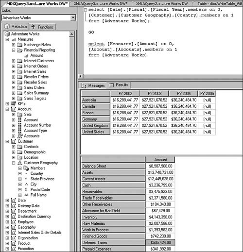 Note Make sure you put a semicolon at the end of the first statement. Also make sure you type GO, not Go because this is case sensitive. How Do I Find a Specific Server Property?The server properties in Analysis Services 2005 are much more numerous than in Analysis Services 2000. They can be counted at well over a hundred. In SQL Management Studio, you can use the Server Properties dialog to edit a property value (see Figure 13-70). Figure 13-70. Analysis Services Properties dialog.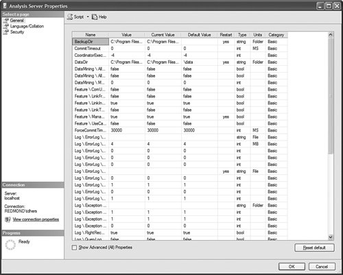 Because of lack of time at the end of the development cycle, the product team was not able to add any search functionality. We realized later on that it would indeed have been a pretty important feature. The reason for this importance is that the property library is read dynamically from the server. This list can change over the course of service packs. So the list is not hard-coded in the tool at all. Also, the list of properties appears with a full categorization-based path of each property. This makes it very hard to sort the property alphabetically and thus search through the list rapidly. As a result, one of the biggest challenges in this dialog is to actually search for and find a specific property. As the author of this dialog I deeply apologize to our audience for overseeing this during our design process and later for missing the window to address this issue during the life cycle of the product. To find a property, my recommendation currently is to edit the MSMSDSRV.INI file that can be found in C:\Program Files\Microsoft SQL Server\MSSQL.2\OLAP\Config, and from which these properties are read, and use the Notepad Find feature to find the property. The server property can be changed directly in the config INI file. If you still want to use the UI, you can just use the INI file to find the path of the property. How Do I Set a Process Option for More than One Object at Once in the Process Object(s) Dialog?Often it can be useful to select multiple objects to process them all at once. By default, the Solution Explorer in BI Development studio enables you to select multiple objects. The Partition tab in the Cube Designer also enables you to select multiple objects. In contrast, in SQL Management Studio the Object Explorer lets you select only one object at a time. Tip To select multiple objects in Solution Explorer, just click on the parent Node and all the dependent objects will be displayed in the Summary report page on the right side. In this Summary tab, the object can be multiselected and an action available in the context menu can be invoked (for example: Process multiple cubes). After the Process dialog has been invoked for multiple objects, they are each represented in a single row. Multiple rows here again can be selected, but now dropping the option list in the Process option column cancels the multiple selection. To change a selection for a set of objects all at once, the user can simply select all the rows simultaneously and then right-click and select one of the available options displayed in the context menu (see Figure 13-71). Figure 13-71. Multiple Selection in Process dialog.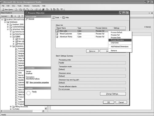 |

 DestinationDimensionName
 ].[
].[
EAN: 2147483647
Pages: 149
- Chapter I e-Search: A Conceptual Framework of Online Consumer Behavior
- Chapter III Two Models of Online Patronage: Why Do Consumers Shop on the Internet?
- Chapter VI Web Site Quality and Usability in E-Commerce
- Chapter VIII Personalization Systems and Their Deployment as Web Site Interface Design Decisions
- Chapter XIV Product Catalog and Shopping Cart Effective Design