SUMMARY DATABASES

Because both statistical databases and OLAP databases are mainly designed for summarization operations, we refer to both with the generic term "summary databases." The concept of "statistical databases" was introduced in the 1980's (Chan & Shoshani, 1981; Shoshani, 1982) and was followed by much activity in this area. The requirements of OLAP were introduced in a white paper by Codd & Associates (1993). This was followed by a paper on the Data Cube (Grey et al., 1996), which is an extension to the relational model to support OLAP databases. It was not apparent initially that both the statistical database and OLAP areas are addressing a similar problem. However, in the article (Shoshani, 1997), we compared statistical databases and OLAP databases in terms of their data models, data structures, and operators. We found the fundamental concepts to be similar, but the work performed in these two domains tended to emphasize different aspects. While much of the work in the statistical database area emphasized conceptual modeling and formalization of operators, the OLAP area emphasized data structures and operational efficiency. However, more recently, more attention is paid to the formal definition of the multidimensional aspects of OLAP databases and their query language (see, for example, Tsois, Karayannidis, & Sellis, 2001; Cabibbo & Torlone, 1997). In this section, we discuss some of the main concepts of summary databases, showing parallels of the statistical database terminology to those of OLAP.

Conceptual Modeling

As mentioned in the introduction, there are two structural features to summary databases: 1) the multidimensional space, and 2) the category hierarchy associated with each dimension. Each dimension (such as "sex" or "age") has a set of categorical values (or categories) associated with it (such as the "sex" categories: "male," "female," and the "age" categories: 1, 2,…, 100). The multidimensional space is simply a cross-product of dimension categories. The categories of a dimension can be further grouped into a category hierarchy (such as grouping "age" into "age groups" of “1–10,…, 91–100).

Initially, each point in the multidimensional space is associated with some object identifier (such as "personID"), as was shown in Figure 1a. As mentioned above, this is referred to as the "base data" or the "microdata." Summary databases are constructed/derived from the microdata by applying a summary operator (such as "count," "sum," "average," etc.) to produce a "summary measure." This operation transforms a "micro database" into a "summary database."

Consider again the example of Figure 1, where we add "projectID" to the employee table. In the customary "relational" notation, this will be represented as: [Employee (personID, age, sex, projectID, salary)]. Note that this notation alone does not represent the fact that there are functional dependencies between Person_ID and each of the attributes age, sex, projectID, and salary. If we use ":" to denote "functional dependency," this may be represented as [personID: age, sex, projectID, salary]. Constructing/deriving a summary database from this micro database amounts to creating a new "summary measure" (or "variable") on the multidimensional space. For example, we can choose to derive a summary database with a summary measure of "average-salary" associated with the multidimensional space (age, sex, projectID). We may use the notation for that as [(age, sex, projectID): average-salary]. That is, there is a functional dependency from the multidimensional space defined by (age, sex, projectID) to average-salary. Thus, every point in this multidimensional space has an average-salary associated with it.

Of course, the summary database can be represented as a table (a relation), such as [salary-info (age, sex, projectID, average-salary)], but the semantics are then lost. The main concept of summary databases is to capture the multidimensional space and the dependency of the summary measure on that space. Further, the concept of a category hierarchy needs to be explicitly captured. This can be done by a "→" notation, such as [age → age-group] or [city → state → region]. For the example above we might group "projectID" into "project-type." Our summary database would then be represented as: [(age → age-group, sex, projectID → project-type): average-salary].

The above notation captures the two main structural concepts as well as the summary measure. In the area of statistical databases, a graphical notation was used to show these concepts explicitly (Shoshani, 1982). Figure 3a represents the example above in that graphical notation, where the "S" node represents a "summary measure," the "X" node represents a "cross-product" of the dimensions underneath it, and the "C" nodes represent category classes. The categories of a "C" node may be further grouped into categories of the "C" node below it. Another graphical notation preferred by some is the Universal Markup Language Notation (UML) where the summary measure is at the bottom of the graph and the categories are at the top (see, for example, Pedersen, Jensen & Dyreson, 1999). This is shown for the same example in Figure 3b.

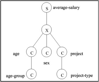
Figure 3a: A Graphical Representation of a Summary Database

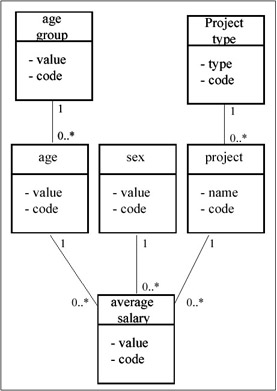
Figure 3b: An Inverted Graphical à Representation Using UML Notation

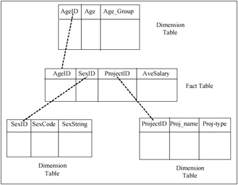
Figure 3c: A Star Schema Representation of the Summary Database

Our purpose in showing the above graphical notations is to emphasize that these are various forms that represent the same concepts. In the OLAP area, relational table structures are used, but additional structure was necessary to capture the concept of a multidimensional "cube" and the category hierarchy structure. In order to represent the semantics of a "cube," a "star schema" is used, where the multidimensional cube and the summary measure are represented in a "fact table" that is placed in the center of the "star," and "dimension tables" represent dimension categories as well as the hierarchical structure of the categories. We show this tabular notation for the example above in Figure 3c. Note that without external labels to the tables, there is no way of telling which is the "fact table" and which are the "dimension tables." Also note that in the fact table there is no way of telling which is the summary measure, except from the meaning of the names of the columns. Similarly, there is no explicit way of telling in the dimension tables that there is a classification hierarchy, except by guessing from the labels of the columns. The reason for this situation is that the tables are devoid of any semantics. Other graph representations used in the literature follow the entity-relationship notation (e.g., Tsois, Karayannidis, & Sellis, 2001; Cabibbo & Torlone, 1998) or other data cube notations (e.g., Lehner, Ruf, & Teschke, 1996).

Supporting Related Information

In practice, the categories involved in the summary databases may have secondary data associated with them. In the above example, a "project-ID" may have "project-description" or "project-deadline" associated with it. Furthermore, projects may belong to city departments, and the cities may have attributes such as "size," "total-budget," and "mayor."

Where in the summary model does such information fit? One solution taken by many authors is to extend the summary model to include additional structures that support associations and even generalization/classification (e.g., Lehner, Ruf, & Teschke, 1996; Sellis, 2000). Another approach is to provide for "links" between an "object" data schema and a "summary" data schema. This approach can also be used in cases where the "object" databases and the "summary" databases can reside on different systems. In this case the links can be supported as a federation of databases using the well-known concepts of "wrappers" and a "mediator." We have investigated this approach in Pedersen, Shoshani, Gu, & Jensen (2000), and built a prototype system on top of the ORACLE relational system and Microsoft's "OLE DB for OLAP" to illustrate its usefulness. This approach can be illustrated in the example shown in Figure 4.

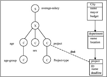
Figure 4: Using Links to Federate "Object" and "Summary" Databases

In this example we show a single link between the category class "project" in the summary database and the "project" object class in the object database. This is a one-to-one link. In general, one can have multiple links set between the database schemas. Also, links can represent other association cardinalities (one-to-many, etc.), or even have attributes defined for the link instances. Once this federation is defined and the links instantiated, it is now possible to ask queries that span both databases. For the example in Figure 4, suppose that the summary database is for all the employees in a particular state. This database is maintained by the state's financial office. Suppose that another "public works" object database shown on the right is maintained by the state's public projects office. One can formulate the query “find Average-Salary by age for all projects in the cities that have a budget greater than $10 million. This query implies that only the projects in departments that belong to cities with a budget greater than $10 million will be selected, and the results summarized over them, as well as over sex.

The linking of databases allows the separation of summary data from other related information. This can be done in a single database system or across a federation. In the example of Figure 4, the separation allows each office to manage its own database, and the federation allows joint queries. For systems that implement OLAP databases as relational tables (such as Microsoft's "OLE DB for OLAP"), "links" are implied when additional tables for the related information are added, but this requires that all the databases are managed by a single system. Also, the semantics of the summary part of the tables and the other information is not explicit. The treatment of summary database semantics explicitly as part of an "object" model is still missing from commercial products. The use of links can facilitate this capability, even if they are applied in a single database system, let alone as a way to define federations between summary and object database systems.

Implied Aggregation

One can take advantage of the structural semantics of summary databases to imply the aggregate operations that need to be performed. This can greatly simplify the query expressions for specifying operations on summary databases. The implied aggregation is based on the multidimensional property, the category hierarchy property, and the "aggregate operator" associated with the summary measure. We discuss first the semantics of the "aggregate measure."

Once a summary database is created, the "summary measure" has an "aggregate operator" (also referred to as "summary operator") associated with it. Typical aggregate operators are "count," "sum," "maximum," "minimum," and "average." For example, the summary measure "population" has the aggregate operator "count" associated with it, and the summary measure "average-income" naturally has the aggregate operator "average" associated with it. We note that in order to support further aggregation with the "average" operator, the system has to carry the "sum" and "count" of the base items involved. More complex operators, such as "mean" and "standard-deviation," can also be calculated by carrying the appropriate base values.

We illustrate the concept of implied aggregation with a simple example. Consider again the summary database of Figure 3. Let's assume the database represents "average-salary-in-California." Recall that it has the following schema: [avg-sal-Cal (age → age-group, sex, projectID → project-type): average-salary], where "avg-sal-Cal" is the name of the database.

Consider the following query applied to this database: "get average-salary for women by project-type." While this seems perfectly understandable to us, there are three implied instructions for performing this query:

1. In calculating the result, aggregate over all ages for each (sex = female, project-type) combination. This is implied because the "age" dimension was NOT mentioned at all in the query.

2. In calculating the result, aggregate over all projects that are in the same project-type. This was implied because of the category hierarchy between "projectID" and "project-type."

3. In calculating the result, use the aggregate operator "average." This is implied because of the default operator associated with the summary measure "average-salary."

As can be seen from this example, the implied aggregation is based on the three structural properties of summary databases: the multidimensionality, the category hierarchy, and the default aggregation operator. As mentioned above this can simplify the query language. We used such a language in Pedersen, Shoshani, Gu, & Jensen (2000). The language is called SumQL, has an SQL format, but takes advantage of the implied aggregation to simplify the query. As an example, the above query is given below as a SumQL query.

   SELECT average-salary   BY_CATEGORY sex, project-type   FROM avg-sal-Cal   WHERE (sex = female) 

Note that joins are not necessary, and the implied aggregation operations ("sum over ages" and "sum over projects") are omitted.

Summarizing category hierarchies requires that these hierarchies are well formed. For example, aggregating "population" from cities to "states" is not well formed, since states contain regions other that cities, such as farmlands, or small towns. However, if we added one fictitious city called "other" to the list of cities, and associated with it all the non-cities population, then we can summarize correctly to the state level. We call the property of being able to correctly aggregate to the next higher category level "summarizability." We studied the summarizability conditions of summary database in Lenz & Shoshani (1997).

Efficiency Considerations

The main efficiency issue in summary databases is how to efficiently compute aggregate operations over the cells of the multidimensional space, and how to extract efficiently subsets of the multidimensional space. There are basically two types of aggregation operations, corresponding to the multidimensional property and the category hierarchy property. These are:

a.1	Aggregating over an entire dimension. This is referred to in the OLAP literature as a "consolidate" operation. For example, in the summary database [population_in_US (state, sex, age): population], aggregating over age to generate [population_in_US (state, sex): population] is a "consolidate" operation over the dimension "age."
a.2	Aggregating over a dimension to a higher level of the category hierarchy. This is referred to in the OLAP literature as a "roll-up" operation. For example, suppose that we have the mapping of "states" to "regions" (such as "west," "mid-west," "south," and "east"), then the summary database [population_in_US (state, sex, age): population] can be rolled-up to produce [population_in_US (region, sex, age): population].

As for selecting efficiently subsets of the multidimensional space, most of the attention in the literature was given to two types of "subset selection" operators:

s.1	Selecting a single value out of a dimension. This is referred to in the OLAP literature as a "slice" operation. For example, selecting only a single state (say "Alabama") for the summary database [population_in_US (state, sex, age): population] will produce [population_in_Alabama (sex, age): population]. Notice that this reduced the database from a three-dimensional database to a two-dimensional database, which is the intuition for the term "slice."
s.2	Selecting a range of values out of a dimension. This is referred to in the OLAP literature as a "dice" operation. For example, selecting only the ages 1–18 (to get only children's population) from the summary database [population_in_US (state, sex, age): population] will produce the multidimensional subset (also referred to as a "sub-cube") [population_of_children_in_US (state, sex, age): population], where age is limited to 1–18. In this case the dimensionality of the sub-cube is the same as the original summary database.

Note that although "slice" can be considered a special case of "dice," they may require support of different data structures and indexes, since they are analogous to performing a single value selection (where hash indexes are most effective for a single attribute) vs. a "range" selection (where tree indexes are most effective for a single attribute). However, in summary databases, multi-attribute indexes are needed for these operations.

There are other operations of interest, such as taking the union of two cubes or disaggregating to lower levels of the category hierarchies, but most of the works published about processing queries efficiently are primarily concerned with the above four operations. As an example for such a cube-query-language (CQL) that supports the above operations and extension to them, see Bauer & Lehner (1997).

Summary query languages combine these four basic operations in various ways. The problem is how to efficiency compute and generate the results for ad-hoc queries involving these operators. The main idea for dealing with this problem is to materialize (pre-compute) sub-cubes. However, just considering the "consolidated" sub-cubes (the operation referred to as operation A.1) is problematic since there are 2ⁿ−1 possible combinations of sub-cubes to consider. For example, a summary database with three dimensions (x,y,z) has sub-cubes with the following dimensions: (x,y,z), (x,y), (x,z), (y,z), (x), (y), (z). A seminal paper addressing this problem was by Harinarayan, Rajaraman, & Ullman (1996). Essentially, the problem they addressed can be formulated as follows: given a limited space (say 20% of the original database size), and the cardinality of each dimension, which sub-cubes should be materialized, given equal probability of all possible ad-hoc queries. They developed an analytic algorithm to determine the optimal selection of sub-cubes to materialize.

Following this work, there were a large number of works that dealt with algorithms that are sensitive to the query patterns or that are better suited for performing update operations. For example, see the paper on dynamic data cubes (Geffner, Agrawal, & El Abbadi, 2000) which also summarizes previous work in this domain.