7.3 Types of Indexes in Oracle Database

---

These are the types of indexes available in Oracle Database.

• Efficient as read-write indexes.

  • BTree (binary tree).

  • Function based.

  • Reverse key.

• Efficient as read-only indexes.

  • Bitmap.

  • Bitmap join.

  • Index-organized table, sometimes useful as read-write indexes.

  • Cluster and hash cluster.

• Domain indexes have a very specific application in an Oracle Database optional add-on and are beyond the scope of this book.

There are also certain attributes of some index types relevant to tuning.

• Ascending or descending.

• Uniqueness.

• Composites.

• Compression.

• Reverse key indexes.

• Unsorted indexes using the NOSORT option.

• Null values.

Let's take a very brief look at index syntax. Then we will proceed to describe each index structure, how they should be used and how they can be tuned without delving too much into physical tuning.

7.3.1 The Syntax of Oracle Database Indexes

Following is a syntax diagram for the CREATE INDEX and ALTER INDEX commands. Since we are in the SQL code tuning section of this book any physical attributes are reserved for possible discussion in Part III on physical and configuration tuning. Parts of the syntax diagram are highlighted to denote parts of Oracle Database index object maintenance relevant to SQL code tuning. Some parts are physical tuning.

CREATE [ UNIQUE | BITMAP ] INDEX [ schema.] index ON      {    [ schema.]table [ alias ] ( column [, column       … ] | expression )    {          [[ NO ] COMPRESS [ n ] ] [ NOSORT | REVERSE ]          [ ONLINE ] [ COMPUTE STATISTICS ] [ TABLESPACE             tablespace ]          [[ NO ] LOGGING ]          [ physical properties ]          [ partitioning properties ]          [ parallel properties ]    } } | CLUSTER [ schema.]cluster { cluster properties } | Bitmap join index clause; ALTER [ UNIQUE | BITMAP ] INDEX [ schema.]index [       [ ENABLE | DISABLE ] [ UNUSABLE ] [ COALESCE ]       [ RENAME TO index ] [[ NO ] LOGGING ] [[ NO ]          MONITORING USAGE ]       [ REBUILD [[ NO ] COMPRESS [ n ] ] [[ NO ] REVERSE ]             [ ONLINE ] [ COMPUTE STATISTICS ] [ TABLESPACE                tablespace ]             [[ NO ] LOGGING ]       ]       [ physical properties ]       [ partitioning properties ]       [ parallel properties ]       [ deallocate unused clause ]       [ allocate extent clause ] ] | CLUSTER [ schema.]cluster { cluster properties };

7.3.2 Oracle Database BTree Indexes

Figure 7.1 shows the internal structure of a BTree index. Note that there are only three layers. Each separate boxed numbered block node in Figure 7.1 represents a block in an Oracle database. A block is the smallest physical unit in an Oracle database. Every read of a datafile will read a single block or more blocks. A unique index scan reading a single row will read the index datafile up to three times and the table once. Three blocks will be read: the root node index block, the second layer index branch block, the index leaf block, and finally the block in the table containing the row using the ROWID pointer stored in the index. Indexes for very small tables may be contained in a single block. All these block references are accessed using ROWID pointers. ROWID pointers are very fast. Unique index hits are the fastest way of accessing data in a database.

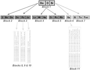
Figure 7.1: An Oracle Database BTree Index

A BTree index does not overflow like other types of indexes. If a block is filled a new block is created and branch nodes are changed or added as required. The parent branch and root node contents could even be adjusted to prevent skewing. Only a change to an indexed table column will change a BTree index. BTree indexes are the best index for obtaining exact row hits, range scans, and changes to the database. The only exception to the overflow rule for a BTree index is where duplicate index values not fitting into a single block can extend into new blocks. This type of overflow is not quite the same as overflow in other index types since other index types do not update index structure "on the fly" as effectively as BTree indexes, if at all.

The following query retrieves index statistics from the USER_INDEXES metadata view, sorted in branch-level order for all the Accounts schema tables. The lower the branch depth level of the BTree the better since less searching through branches is required. In general, any index will become less efficient as it becomes larger and contains more duplicates.

• Branch level 0 indexes are all small static data tables.

• Branch level 1 indexes are dynamic tables where foreign or alternate key indexes are usually on unique integer identifier column values.

• Branch level 2 indexes are very large tables or low cardinality, nonunique foreign key indexes.

  SELECT table_name,index_name,num_rows "Rows"       ,blevel "Branch",leaf_blocks "LeafBlocks" FROM user_indexes WHERE index_type = 'NORMAL' AND num_rows > 0 ORDER BY blevel, table_name, index_name;                                                              Leaf TABLE_NAME      INDEX_NAME              Rows  Branch  Blocks -------------   -------------------     ----  ------  ------ CATEGORY        AK_CATEGORY_TEXT          13       0       1 CATEGORY        XPKCATEGORY               13       0       1 COA             XFK_COA_SUBTYPE           55       0       1 COA             XFK_COA_TYPE              55       0       1 COA             XPKCOA                    55       0       1 POSTING         XFK_POSTING_CRCOA#         8       0       1 POSTING         XFK_POSTING_DRCOA#         8       0       1 POSTING         XPKPOSTING                 8       0       1 STOCK           XFK_STOCK_CATEGORY       118       0       1 STOCK           XPKSTOCK                 118       0       1 SUBTYPE         XPKSUBTYPE                 4       0       1 TYPE            XPKTYPE                    6       0       1 CASHBOOK        XPKCASHBOOK           188185       1     352 CASHBOOKLINE    XFK_CBL_CHEQUE        188185       1     418 CASHBOOKLINE    XFK_CBL_TRANS         188185       1     418 CASHBOOKLINE    XPKCASHBOOKLINE       188185       1     423 CUSTOMER        AK_CUSTOMER_NAME        2694       1      17 CUSTOMER        AK_CUSTOMER_TICKER      2694       1      12 CUSTOMER        XPKCUSTOMER             2694       1       5 ORDERS          XFK_ORDERS_CUSTOMER    31935       1      67 ORDERS          XFK_ORDERS_CUSTOMER   140369       1     293 ORDERS          XFK_ORDERS_TYPE       172304       1     313 ORDERS          XPKORDERS             172304       1     323 STOCK           AK_TEXT                  118       1       2 STOCKSOURCE     XFK_STOCKSOURCE_STOCK  12083       1      24 STOCKSOURCE     XFK_STOCKSOURCE_       12083       1      26                    SUPPLIER STOCKSOURCE     XPKSUPPLIER_STOCK      12083       1      46 SUPPLIER        AK_SUPPLIER_NAME        3874       1      27 SUPPLIER        AK_SUPPLIER_TICKER      3874       1      17 SUPPLIER        XPKSUPPLIER             3874       1       7 TRANSACTIONS    XFX_TRANS_CUSTOMER     33142       1      70 TRANSACTIONS    XFX_TRANS_ORDER       173511       1     386 TRANSACTIONS    XFX_TRANS_SUPPLIER    155043       1     324 TRANSACTIONS    XFX_TRANS_TYPE        188185       1     341 TRANSACTIONS    XPKTRANSACTIONS       188185       1     378 CASHBOOK        XFK_CB_CRCOA#         188185       2     446 CASHBOOK        XFK_CB_DRCOA#         188185       2     446 GENERALLEDGER   AK_GENERALLEDGER_1    752744       2    4014 GENERALLEDGER   AK_GL_DTE             752744       2    1992 GENERALLEDGER   XFK_GL_COA#           752744       2    1784 GENERALLEDGER   XPKGENERALLEDGER      752744       2    1425 ORDERSLINE      XFK_ORDERLINE_ORDER   540827       2    1201 ORDERSLINE      XFK_ORDERLINE_SM      540827       2    1204 ORDERSLINE      XPKORDERSLINE         540827       2    1215 STOCKMOVEMENT   XFK_SM_STOCK          570175       2    1124 STOCKMOVEMENT   XPKSTOCKMOVEMENT      570175       2    1069 TRANSACTIONS    XFX_TRANS_CRCOA#      188185       2     446 TRANSACTIONS    XFX_TRANS_DRCOA#      188185       2     446 TRANSACTIONS-   XFK_TRANSLINE_SM      570175       2    1270    LINE TRANSACTIONS-   FK_TRANSLINE_TRANS    570175       2    1267    LINE TRANSACTIONS-   XPKTRANSACTIONSLINE   570175       2    1336    LINE

That's enough about BTree indexes for now. We will cover some nonphysical tuning aspects shortly. Let's take a look at the other Oracle Database index types.

7.3.3 Read-Only Indexing

Read-only indexes are generally applicable to reporting and data warehouse databases. This book is not intended as a data warehouse book. However, these types of indexes can be used in online and client-server databases with one restriction: the more table changes are made the more often these types of indexes must be rebuilt. There are a number of big issues with respect to non-BTree indexes.

• They can be extremely fast in proper circumstances. Read-only indexes are designed for exactly that and are built to perform well when reading data.

• Two issues are associated with read-only indexing when making changes to tables.

  • When changed, these indexes will generally overflow and rapidly become less efficient. Future read access requiring overflowed rows will search outside the original index structure. The point of an index is searching of preordered physical space.

  • The more changes made, the slower future changes will be.

Let's take a brief look at the different types of read-only indexes.

Bitmap Indexes

A bitmap index stores a value of 0 or 1 for a ROWID. The ROWID points to a row in a table. In Figure 7.2 a bitmap index is created on a column containing codes for states.

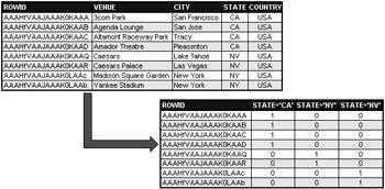
Figure 7.2: A Bitmap Index

There are some things to be remembered when considering using bitmap indexes.

• In general bitmaps are effective for single-column indexes with low cardinality.   Low cardinality implies very few different values. However, bitmap indexes can perform relatively well with thousands of different values. The size of a bitmap index will be smaller than that of a BTree and thus search speed is increased by searching through less physical space.

• Bitmap indexes are much faster than BTree indexes in read-only environments.

• Probably the most significant performance issue with bitmap indexes is that unlike BTree indexes bitmaps will lock at the block level rather than the row level. Since a bitmap index will have more index entries per block due to less space used, it becomes even more likely that locking will cause performance problems with UPDATE and DELETE commands. UPDATE and DELETE commands require exclusive locks.

• Bitmap indexes should not be used to create composite-column indexes. Composite values are likely to have many different values (high cardinality). If composite-column indexes are required simply create multiple single-column bitmap indexes on each column. SQL WHERE clause filtering in Oracle Database can match multiple single-column bitmap indexes in the same query, in any order.

• Bitmap indexes may be subject to overflow. Quite often bitmaps are used in large data warehouse databases where changes are not made to tables other than complete reloads.

  Tip 

  Traditionally any index type other than a BTree index involves overflow. Overflow involves links between blocks where values cannot fit into previously reserved index space. Overflow is detrimental to performance.

Like BTree indexes bitmap indexes should probably be regularly rebuilt. However, for large databases regular bitmap index rebuilds can consume more time than is acceptable. Therefore bitmap indexes are most appropriate for large, low cardinality, read-only, static or transactional data tables.

Let's do some experimenting and show that bitmap indexes are faster than BTree indexes.

Are Bitmap Indexes Faster than BTree Indexes?

The Transactions table contains a column called type having two possible values representing a customer or a supplier-based transaction.

SQL> SELECT type "Type", COUNT(type) FROM transactions   GROUP BY type;     T  COUNT(TYPE) -  ----------- P       175641 S        61994

I am going to create two temporary copies of the Transactions table. One will have a BTree index on the type column and the other a bitmap index.

CREATE TABLE btree_table AS SELECT * FROM transactions; CREATE INDEX btree_index ON btree_table(type) COMPUTE    STATISTICS; CREATE TABLE bitmap_table AS SELECT * FROM transactions; CREATE BITMAP INDEX bitmap_index ON bitmap_table(type)       COMPUTE STATISTICS;

Since we will be using the EXPLAIN PLAN command to demonstrate we need to generate statistics for the new objects.

ANALYZE TABLE btree_table COMPUTE STATISTICS; ANALYZE TABLE bitmap_table COMPUTE STATISTICS;

Looking at the query plans we can see that accessing the bitmap index is faster than using the BTree index. I used hints in order to force usage of the required indexes. The type = 'P' comparison accesses just shy of 75% of the table. The Optimizer will do a full table scan without the hints.

EXPLAIN PLAN SET statement_id='TEST' FOR       SELECT /*+ INDEX(btree_table, btree_index) */ *       FROM btree_table WHERE type = 'P';     Query                                 Cost     Rows     Bytes -----------------------------------   ----   ------   ------- SELECT STATEMENT on                   1347    94093   3387348  TABLE ACCESS BY INDEX ROWID on     BTREE_TABLE                        1347    94093   3387348   INDEX RANGE SCAN on BTREE_INDEX      171    94093     EXPLAIN PLAN SET statement_id='TEST' FOR       SELECT /*+ INDEX(bitmap_table, bitmap_index) */ *       FROM bitmap_table WHERE type = 'P';     Query                                 Cost     Rows     Bytes -----------------------------------   ----   ------   ------- SELECT STATEMENT on                    806    94093   3387348  TABLE ACCESS BY INDEX ROWID on        806    94093   3387348   BITMAP_TABLE   BITMAP CONVERSION TO ROWIDS on    BITMAP INDEX SINGLE VALUE on      BITMAP_INDEX 

Timing the SQL statements we can see again that accessing the bitmap is much faster. A different-sized table with a different selection may have had a more significant difference.

SQL> SELECT COUNT(*) FROM (   2 SELECT /*+ INDEX(btree_table, btree_index) */ *   3 FROM btree_table WHERE type = 'P');        COUNT(*) -----------       33142     Elapsed: 00:00:01.01     SQL> SELECT COUNT(*) FROM (   2 SELECT /*+ INDEX(bitmap_table, bitmap_index) */ *   3 FROM bitmap_table WHERE type = 'P');        COUNT(*) -----------       33142     Elapsed: 00:00:00.00 

Bitmap indexes can be significantly faster than BTree indexes. Costs in the two previous query plans decreased for the bitmap index from 1347 to 806, a 40% decrease in cost.

Tip 

During the period in which these query plans were generated no

DML type changes were made to the two new tables.

Let's clean up by dropping the tables. Dropping the tables will drop the attached indexes.

DROP TABLE btree_table; DROP TABLE bitmap_table;

Bitmap Index Locking

As already stated there is one particular case I remember where many bitmap indexes were used. The database was in excess of 200 Gb and had a fairly large combination online and reporting production database. When one of the bitmaps was changed to a BTree index, a process taking 8 h to run completed in less than 3 min. Two possible causes would have been bitmap index block level locks as a result of heavy DML activity or, secondly, perhaps uncontrollable bitmap index overflow.

Using Composite Bitmap Indexes

Let's do query plans and some speed checking with composite-column indexing.

CREATE TABLE btree_table AS SELECT * FROM stockmovement; CREATE INDEX btree_index ON btree_table    (stock_id,qty,price,dte)       COMPUTE STATISTICS; CREATE TABLE bitmap_table AS SELECT * FROM stockmovement; CREATE BITMAP INDEX bitmap_index ON bitmap_table       (stock_id,qty,price,dte) COMPUTE STATISTICS;

Since we will be using the EXPLAIN PLAN command to demonstrate we need to generate statistics for the new objects.

ANALYZE TABLE btree_table COMPUTE STATISTICS; ANALYZE TABLE bitmap_table COMPUTE STATISTICS;

Start with query plans using the EXPLAIN PLAN command.

EXPLAIN PLAN SET statement_id='TEST' FOR       SELECT /*+ INDEX(btree_table, btree_index) */ *       FROM btree_table       WHERE stock_id IN (SELECT stock_id FROM stock)       AND qty > 0       AND price > 0       AND dte < SYSDATE;     Query                                 Cost     Rows     Bytes -----------------------------------   ----   ------   ------- SELECT STATEMENT on                  10031    16227    105675  TABLE ACCESS BY INDEX ROWID on     BTREE_TABLE                          85      138      3036   NESTED LOOPS on                    10031    16227    105675    INDEX FULL SCAN on XPK_STOCK          1      118       354    INDEX RANGE SCAN on BTREE_INDEX      20      138     EXPLAIN PLAN SET statement_id='TEST' FOR       SELECT /*+ INDEX_COMBINE(bitmap_table, bitmap_index) */ *       FROM bitmap_table       WHERE stock_id IN (SELECT stock_id FROM stock)       AND qty > 0       AND price > 0       AND dte < SYSDATE;     Query                                 Cost     Rows     Bytes -----------------------------------   ----   ------   ------- SELECT STATEMENT on                   7157    16227    405675  NESTED LOOPS on                      7157    16227    405675   TABLE ACCESS BY INDEX ROWID on      7156    16227    356994    BITMAP CONVERSION TO ROWIDS on     BITMAP INDEX FULL SCAN on       BITMAP_INDEX  INDEX UNIQUE SCAN on XPK_STOCK                   1         3

Now some speed testing.

SQL> SELECT COUNT(*) FROM(   2 SELECT /*+ INDEX(btree_table, btree_index) */ *   3 FROM btree_table   4 WHERE stock_id IN (SELECT stock_id FROM stock)   5 AND qty > 0   6 AND price > 0   7 AND dte < SYSDATE);        COUNT(*) -----------      115590     Elapsed: 00:00:00.09     SQL> SELECT COUNT(*) FROM(   2 SELECT /*+ INDEX(bitmap_table, bitmap_index) */ *   3 FROM bitmap_table   4 WHERE stock_id IN (SELECT stock_id FROM stock)   5 AND qty > 0   6 AND price > 0   7 AND dte < SYSDATE);        COUNT(*) -----------      115590     Elapsed: 00:00:00.02 

We can see that even a composite bitmap index is faster than a composite BTree index. However, the cost decrease is 10,031 to 7,157, only a 30% decrease in cost. It could probably be concluded that composite bitmap indexes do not perform as well as single-column bitmap indexes.

Tip 

During the period in which these query plans were generated no DML type changes were made to the two new tables.

Now let's break the bitmap index into separate single-column indexes, run the query plan and timing tests again and see if we get a performance improvement over the composite bitmap index. Drop the previous version of the bitmap index and create four separate bitmap indexes.

DROP INDEX bitmap_index; CREATE BITMAP INDEX bitmap_index _stock _id ON bitmap table    (stock id); CREATE BITMAP INDEX bitmap_index_qty ON bitmap_table(qty); CREATE BITMAP INDEX bitmap_index_price ON bitmap_table(price); CREATE BITMAP INDEX bitmap_index_dte ON bitmap_table(dte);

Note that the hint has changed. The INDEX_COMBINE hint attempts to force usage of multiple bitmap indexes.

EXPLAIN PLAN SET statement_id='TEST' FOR       SELECT /*+ INDEX_COMBINE(bitmap_table) */ * FROM          bitmap_table       WHERE stock_id IN (SELECT stock_id FROM stock)       AND qty > 0       AND price > 0       AND dte < SYSDATE;     Query                                 Cost     Rows     Bytes -----------------------------------   ----   ------   ------- SELECT STATEMENT on                   1004    16226    405650  NESTED LOOPS on                      1004    16226    405650   TABLE ACCESS BY INDEX ROWID on     BITMAP_TABLE                      1004    16226    356972    BITMAP CONVERSION TO ROWIDS on     BITMAP AND on      BITMAP MERGE on       BITMAP INDEX RANGE SCAN on        BITMAP_INDEX_DTE      BITMAP MERGE on       BITMAP INDEX RANGE SCAN on        BITMAP_INDEX_QTY      BITMAP MERGE on       BITMAP INDEX RANGE SCAN on        BITMAP_INDEX_PRICE  INDEX UNIQUE SCAN on XPK_STOCK                   1         3

The cost difference between the composite bitmap index and the single-column bitmap indexes has increased significantly. Using single-column bitmap indexes is much faster than using composite bitmap indexes.

Tip 

During the period in which these query plans were generated no DML type changes were made to the two new tables.

Now let's clean up.

DROP TABLE btree_table; DROP TABLE bitmap_table; 

Do Bitmap Indexes Overflow?

In the previous examples creating the indexes after creating and populating the tables built the indexes in the most efficient way. Now I am going to create a bitmap index in a slightly less appropriate place on a column with lower cardinality. The purpose here is to demonstrate the potential deterioration of bitmap indexes due to overflow. Following is a count of the rows of repeated values of the GeneralLedger.COA# column. The total row count is currently 1,045,681 rows.

SQL> SELECT coa#, COUNT(coa#) FROM generalledger GROUP BY    coa#;     COA#    COUNT(COA#) -----   ----------- 30001        377393 40003        145447 41000        246740 50001        203375 50028             1 60001         72725

Firstly, we need to do a query plan for the current existing BTree index on the COA# column foreign key BTree index.

EXPLAIN PLAN SET statement_id='TEST' FOR       SELECT /*+ INDEX(generalledger, xfk_coa#) */ *       FROM generalledger WHERE coa# = '60001';     Query                                 Cost     Rows     Bytes -----------------------------------   ----   ------   ------- SELECT STATEMENT on                   3441   177234   4076382  TABLE ACCESS BY INDEX ROWID on     GENERALLEDGER                      3441   177234   4076382   INDEX RANGE SCAN on XFK_COA#         422   177234

Now I will change the foreign key index to a bitmap, generate statistics and run the EXPLAIN PLAN command again. Clearly the bitmap is faster than the BTree index.

DROP INDEX xfk_coa#; CREATE BITMAP INDEX xfk_coa#_bitmap ON generalledger(coa#)       COMPUTE STATISTICS; ANALYZE TABLE generalledger COMPUTE STATISTICS;     EXPLAIN PLAN SET statement_id='TEST' FOR       SELECT /*+ INDEX(generalledger, xfk_coa#_bitmap) */ *       FROM generalledger WHERE coa# = '60001';     Query                                 Cost     Rows     Bytes -----------------------------------   ----   ------   ------- SELECT STATEMENT on                   1707   177234   4076382  TABLE ACCESS BY INDEX ROWID on       1707   177234   4076382    GENERALLEDGER   BITMAP CONVERSION TO ROWIDS on    BITMAP INDEX SINGLE VALUE on       XFK_COA#_BITMAP 

Notice how the cost of using the bitmap index is much lower than that of using the BTree index.

In the next step I restart my database and begin processing to execute a large amount of concurrent activity, letting it run for a while. The objective is to find any deterioration in the bitmap index due to excessive DML activity. The row count for the GeneralLedger table is now 10,000 rows more than previously.

ANALYZE TABLE generalledger COMPUTE STATISTICS; ANALYZE INDEX xfk_coa#_bitmap COMPUTE STATISTICS;     EXPLAIN PLAN SET statement_id='TEST' FOR       SELECT /*+ INDEX(generalledger, xfk_coa#_bitmap) */ *       FROM generalledger WHERE coa# = '60001';     Query                                 Cost     Rows     Bytes -----------------------------------   ----   ------   ------- SELECT STATEMENT on                   1729   178155   4097565  TABLE ACCESS BY INDEX ROWID on       1729   178155   4097565    GENERALLEDGER   BITMAP CONVERSION TO ROWIDS on    BITMAP INDEX SINGLE VALUE on       XFK_COA#_BITMAP 

We can see from the two previous query plans that the cost of using the bitmap index has decreased by over 1% after adding around 10,000 rows to the GeneralLedger table. Now I will run the same highly concurrent DML commands and add some more rows to the GeneralLedger table, only this time we will change the bitmap index back to a BTree index and compare the relative query cost deterioration.

DROP INDEX xfk_coa#_bitmap; CREATE INDEX xfk_coa# ON generalledger(coa#); 

Once again I have executed my concurrent processing and added another 10,000 rows to the GeneralLedger table. This time the BTree index is back in place and there is no longer a bitmap index. When processing is complete we analyze statistics and run the EXPLAIN PLAN command again.

ANALYZE TABLE generalledger COMPUTE STATISTICS; ANALYZE INDEX xfk_coa# COMPUTE STATISTICS;     EXPLAIN PLAN SET statement_id='TEST' FOR       SELECT /*+ INDEX(generalledger, xfk_coa#) */ *       FROM generalledger WHERE coa# = '60001';     Query                                 Cost     Rows     Bytes -----------------------------------   ----   ------   ------- SELECT STATEMENT on                   3466   178155   4097565  TABLE ACCESS BY INDEX ROWID on     GENERALLEDGER                      3466   178155   4097565   INDEX RANGE SCAN on XFK_COA#         425   178155

The increase in cost is slightly below 1% for the BTree index. This is unexpected. Where INSERT statements are concerned bitmap indexes are not subject to much overflow on this scale. At a much larger scale the situation may be very different.

Bitmap Join Indexes

A bitmap join index is simply a bitmap containing ROWID pointers of columns or keys used in the join from the tables joined together. The index is created using an SQL join query statement.

Clusters

A cluster is quite literally a cluster or persistent "joining together" of data from one or more sources. These multiple sources are tables and indexes. In other words, a cluster places data and index space rows together into the same object. Obviously clusters can be arranged such that they are very fast performers for read-only data. Any type of DML activity on a cluster will overflow. Rows read from overflow will be extremely heavy on performance. Clusters are intended for data warehouses.

A standard cluster stores index columns for multiple tables and some or all nonindexed columns. A cluster simply organizes parts of tables into a combination index and data space sorted structure. Datatypes must be consistent across tables.

Hash Clusters

A hash cluster is simply a cluster indexed using a hashing algorithm. Hash clusters are more efficient than standard clusters and are even more appropriate to read-only type data. In older relational databases hash indexes were often used against integer values for better data access speed. If data was changed the hash index had to be rebuilt.

Sorted Hash Clusters

 Oracle Database 10 Grid   A hash cluster essentially breaks up data into groups of hash values. Hash values are derived from a cluster key value forcing common rows to be stored in the same physical location. A sorted hash cluster has an additional performance benefit for queries, accessing rows in the order in which the hash cluster is ordered: thus the term sorted hash cluster.

Index-Organized Tables

A cluster is a join of more than one table. An index-organized table is a single table, physically organized in the order of a BTree index. In other words, the data space columns are added into the index structure leaf blocks of a binary tree. An index-organized table is effectively a BTree table where the entire table is the index. Block space is occupied by both data and index values. Much like clusters the sorted structure of an index-organized table is not usually maintained efficiently by DML activity. Any changes to any of the columns in the table will affect the index directly because the table and the index are one and the same thing. It is likely that any DML activity will cause serious performance problems due to overflow and skewing. On the contrary, there are reports of good performance gains using index-organized tables in OLTP type databases. However, I am currently unaware of exactly how these tables are used in relation to DML activity.

---