The Second Dimension: Definition of Thresholds for BCWS

The definition of thresholds for BCWS should be statistically defined. The thresholds cannot be defined arbitrarily as some percentage of allowable variations, agreed to between parties in the contract. Only a quantitative evaluation of it will make the EVM process seamlessly applicable to all applications. So effectively, the process will have a built in "insensitivity." As long as the cost and schedule deviations are within the thresholds or tolerance lines, no specific corrective action is warranted. However, if a deviation crosses the threshold or tolerance lines, a full investigation is required.

Statistical Quality Control

Development of such threshold and tolerance lines can be derived from the basic principles of Statistical Quality Control (SQC) or the Statistical Control Chart theory in general. Control charts were developed as a technique for ensuring that a process remained in statistical control, but not necessarily for ensuring that every item produced was within the tolerance limits set by the specifications. Consider a process that produces items, one of whose dimensions are of primary importance. Statistical control is achieved if the items are produced with a constant mean and variance. The variance is said to be due to non-assignable causes. If the mean level of the dimension moves away from the original mean or if the variance alters by a significant amount, the process is said to have gone out of control. Investigation may also arise if a trend appears, if an unusually large number of observations are above or below the central value, or if several observations are near a control limit.

So the basic concept is that all processes, outputs, and systems exhibit variability. No two things are exactly the same. Schewart refers to the sources of variability as chance and assignable causes and Deming calls them common or special causes. What control charts do is separate the signal of variability due to assignable causes, from the background noise of variability due to chance causes. When chance causes are only playing, the variation follows known patterns of statistical distributions. If a set of data is analyzed and the pattern of variation of data is shown to conform to such statistical patterns that are produced by chance, we can assume that only chance or common cause is operating on the system. In such a situation, a process is said to be under statistical control (Levine et al. 1995). To construct a control chart, we require an estimate of central tendency—the mean—and an estimate of variability—the standard deviation.

According to schewart control charts, the means of each sample n are distributed normally with the mean m and

• R = sample range

• dn = constant for given sample size n

• n = sample size.

Using the fact that a variable which is normally distributed has 99.8 percent of it's values lying less than 3.09 standard deviations from it's mean, it is expected that 99.8 percent of the sample means would lie between m(mean) − 3.09s and m(mean)+3.09s,

These are the lower and upper action limits. Again using the properties of the normal distribution, it may be expected that 95 percent of the sample means would lie between m(mean) + 1.96s and m(mean) − 1.96s. These values are known as the lower and upper warning limits.

Application to Costs

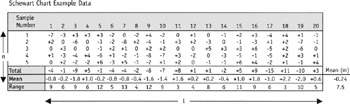
When we try and apply this to costs, the first thing to understand is that cost as a standard for control cannot be a specific value, it has to take the form of a frequency diagram—from which the limits of variation can be determined. If we extend a similar analogy of the Schewart chart method to the various costs constituting a reporting period, we realize that there is a distinct difference. Unlike the Schewart chart methods in the production industry, the problem with cost distribution over a period of time is that what is monitored is not the mean of the costs of the different activities, but their sum total. Table 1, which is a small example of the calculation of various limits, illustrates the point. Hence the formula used for deriving the control limits in Schewart control charts needs to be modified.

In Table 1, the mean of the "I" observations is m, and each of these "I" observations is the mean of sample size n. The mean m has to be modified to form the sum of the "I" observations.

Adding such frequencies whose mean is m, the formula for control limits becomes:

Similarly, the warning limits get modified to:

Since this method considers the ranges of the sample size n, it is important that the various ranges are of compatible order, so that the mean range of the n samples has a significance. This seems to be ideal when the constituent costs are from similar or homogeneous activities, indicating the same order of the quantity of work involved. Activities from the same or similar work package are good examples. Say RCC work in floors one to ten, when the floor sizes are similar. Let's call this Method 1. However, when dealing with non-homogeneous activities or when summing up through various work packages of dissimilar nature, it is better to add up the various variances rather than considering the mean range of samples.

So, the control limits will be:

Let's call this Method 2.

Example Project

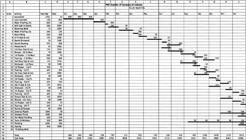
The example project in Table 2 shows activities and their quantities and costs distributed monthly. The cumulative total of these costs when plotted on a time versus cost graph will constitute the initial BCWS. In order to find the threshold limits, each of these costs have to be distributed as a frequency. We need to make a frequency diagram of sample size n. We can consider normal distributions with a 95 percent level of confidence and start with a positive or negative 15 percent variation on either side of a mean—the point estimate. So each cost estimate is made into a sample size of three, with a lower and an upper limit estimated at 95 percent confidence (Table 3). So in our calculations n will be equal to three and "1" will be varying in different months. If a month has five activities in it, "1" will be equal to five, and if it has two, "1" will be equal to two.

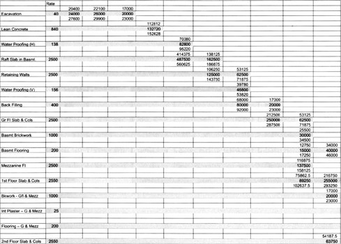
Table 4 shows part of a worksheet that calculates the action limits for cumulative costs in different months. The cumulative mean range of a month is the mean of all component ranges from the beginning of the project until that month. This reflects Method 1.

Table 4: Method 1

Total + 3@l (s/@n)	839668.9	1019615	997364.7	579772.4	1306722	875223.8	60600.17
Cum	5318615	6338230	7335595	7915367	9222090	10097313	10157914
1a from Ranges - R1	1875	15000	26775	2835	1575	16200	15000
R2	15000	13837.5	13680	25200	1417.5	19845
R3	5940	13680	99375	13680	27412.5	30000
R4	2625	2730	4500	1417.5	16200	102000
R5	12300	99375	21600	4500	4500	13200
R6	78000	21600		19845	45360
R7	21600			24000	18630
R8				30000	24000
R9					67500
R10					60000
Cum Values
Cum Mean R	26818.89	26948.38	27626.38	25783.17	25920.09	26668.57	27060.75
s=(Cumm R)/(1.693*@n)	9145.24	9189.397	9420.596	8792.06	8838.752	9093.981	9227.716
3s@l	162145.1	176436.4	191614.9	193601.2	212130	224803.2	229770.1
Cum + 3s @l	3291015	3859381	4427660	4834571	5741750	6238423	6293390
Cum − 3s @l	2966725	3506509	4044430	4447369	5317490	5788817	5833850
Note: All "@" Should Be Read as "sq root"

Table 5 shows a part of a worksheet that calculates the action limits for cumulative costs in different months, by Method 2. The cumulative grand variance of a month adds all component variances from the beginning of the project until that month.

Table 5: Method 2

CV10					225000000
Grand Variance	435783740.6	684563895.7	704140228.1	170143934.8	760967599.2	758406501.6	14062500
For Cum Sigmas Cum Grand Variance	3574936580	4259500476	4963640704	5133784639	5894752238	6653158739	6667221239
Cum Std Dev (Sigma)	59790.77337	65264.8487	70453.10997	71650.43363	76777.28986	81566.89733	81653.05407
3 Sigma	179372.3201	195794.5461	211359.3299	214951.3009	230331.8696	244700.692	244959.1622
Cum Total +3 Sigma	3308242.32	3878739.546	4447404.33	4855921.301	5759951.87	6258320.692	6308579.162
Cum Total −3 Sigma	2949497.68	3487150.454	4024685.67	4426018.699	5299288.13	5768919.308	5818660.838
2 Sigma	119581.5467	130529.6974	140906.2199	143300.8673	153554.5797	163133.7947	163306.1081
Cum Total + 2 Sigma	3248451.547	3813474.697	4376951.22	4784270.867	5683174.58	6176753.795	6226926.108
Cum Total −2 Sigma	3009288.453	3552415.303	4095138.78	4497669.133	5376065.42	5850486.205	5900313.892

Figure 2, shows the graphical BCWS drawn as a cumulative S curve, obtained by the Method 1. Figure 3 shows the graphical BCWS curve, obtained by the Method 2. In our example project, both turned out more or less similar. The most important conclusion from this exercise emerged in the finding that although we started with a 15 percent allowance in variation of each of the component costs (with a 95 percent confidence), the final allowable variance in the total cost worked out at 4 percent only, for a 99 percent confidence interval.

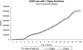
Figure 2: Method 1 from Component Ranges

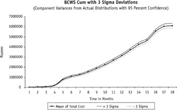
Figure 3: Method 2 from Component Variances

This looks like too narrow a band for all practical purposes as shown in Figures 2 and 3. However, just the fact that the action limits are mostly like parallel curves on both sides of the BCWS indicates that it has maintained the same distance from a higher cumulative cost (at the end of the project) as from a lower cumulative cost (at the initial stages of the project). This means a lower percentage of variation for the higher costs than for the lower costs. This also brings us to the point where we need to optimize the allowable variations in the components and the total cost by using a sensitivity analysis. It turned out to be an iterative process, where we determined an end contingency and distributed it. The most important tool was the understanding that a 10 percent contingency to the total cost allowed us to have a much bigger contingency of the component costs.