Analysis of the Decision Tree

First, we have some notation. With T as the general decision tree for a project, let P denote a path in T, where a path is a sequence of edges of T, from the root of T to a tip (terminal point) of T. What is the duration of the path P? Clearly this will be the sum of the durations of the tasks plus any lead-time delays along the path. Determining the delays requires some calculations, which we consider next.

Observe that lead-time delays can only occur for tasks that are crashed. Along a path P in T we start with task A and then iteratively consider B, and then C, and so forth. Suppose that A is crashed along P. If the lead-time for task A is positive, then A's lead-time delay equals its lead-time (since we assume that the project starts as soon as possible). Otherwise, A's lead-time delay is zero. In general, for any crashed task j on path P we compute the elapsed time along P from the point where the crash decision is made until the time that the predecessor tasks of j are completed. This elapsed time is, of course, simply the sum of the durations of the events (including any lead-time delays) along the path from the point of the crash decision to (and including) the immediate predecessors of task j. If the lead-time of task j is greater than this elapsed time, then the lead-time delay equals the difference "lead-time – elapsed time." Otherwise, we say that the lead-time delay is zero. In Figure 4, observe that the lead-time delay of task B on path nineteen (the 19^th path from the top) is one. Here the corresponding elapsed time is five and the lead-time of B is six, so that the lead-time delay is 6 − 5 = 1.

We now consider a companion concept of lead-time delay. Again, as above, for each crashed task j along P we iteratively compute the difference between elapsed time and lead-time. However, if the lead-time is less than the elapsed time, the difference (elapsed lead-time) is called the lead-time slack of j along P. If the lead-time slack is not less than the elapsed time, then we define the lead-time slack as zero. For a task not crashed along P we say that its lead-time slack along P is ∇. Let S(j,P) denote the lead-time slack of task j along P. As an illustration, observe that the lead-time slack of task C along path five in Figure 4 is five since the elapsed time is eleven and the lead-time is six. Also note that for any task j, at most one of lead-time delay and lead-time slack in positive.

For given lead-times, the duration at each terminal point on the tree is simply the sum of the durations of the tasks along the corresponding path. This duration may result is some indirect or penalty cost, which can be added to the total cost of crashing tasks along the corresponding path. Then, the expected cost of the project can be determined by doing the standard backward folding of the decision tree T, yielding optimal decisions at the decision nodes. (Of course, some decision nodes may have alternative optimal decisions.)

Consider an optimal solution to the decision problem where exactly one branch out of each decision node is specified. Let T* denote a strategy subtree consisting of those paths P where all decision branches on each such path correspond to this optimal solution. Observe that T* specifies the optimal decision to be selected at each decision point that can be attained with a positive probability. To illustrate, consider the following example.

Suppose that indirect costs are related to project duration as given in Figure 5. It can be shown that the optimal solution in this situation is A no, B no, and C no at all decision points, except for the case where both A NL and B NL occur. In that case, we choose C yes. The optimal strategy subtree T* for this is the union of paths 1, 2, 3, 4, 7, 8, 11, and 12 in Figure 4. The expected cost of this strategy is $407.50.

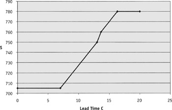
Figure 5: Project Cost versus Activity C Lead-Time

Consider some path PΛTM*. We now define the minimum lead-time slack of task j, denoted S(j), as:

S(j) = Min{S(j,P) for PΛT*}

Note that S(j) gives the upper limit of increase in the lead-time in task j before any increase in the cost of the project will be incurred. In Figure 2 for task C the minimum lead-time slack is five since only two paths in T* have a crashed duration for C (paths eleven and twelve in Figure 4) and the slack there is five. Thus, the cost impact of an increase in the lead-time of task C is zero up to an increase of five.