Using Formulas
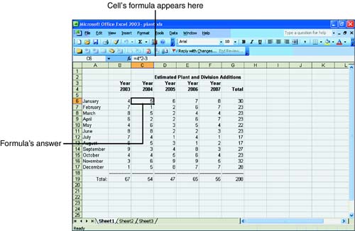
| Without formulas , Excel would be little more than a simple row- and column-based word processor. When you use formulas, however, Excel becomes an extremely powerful time-saving planning, budgeting, and general-purpose financial tool. On a calculator, you typically type a formula and then press the equal sign to see the result. In contrast, all Excel formulas begin with an equal sign. For example, the following is a formula: =4*2-3 The asterisk is an operator that denotes the times sign ( multiplication ). This formula requests that Excel compute the value of 4 multiplied by 2 minus 3 to get the result. When you type a formula and press Enter or move to another cell , Excel displays the result and not the formula on the worksheet. As Figure 7.4 shows, the answer 5 appears on the worksheet, and you can see the cell's formula contents right on the formula bar area. When entering a formula, as soon as you press the equal sign, Excel shows your formula on the formula bar as well as in the active cell. If you click the formula bar and then enter your formula, the formula appears in the formula bar as well as in the active cell. By first clicking the formula bar before entering the formula, however, you can press the left- and right-arrow keys to move the cell pointer left and right within the formula to edit it. When entering long formulas, this formula bar's editing capability helps you correct mistakes that you might type. Figure 7.4. Excel displays a formula's result on the worksheet. Excel's Primary Math OperatorsTable 7.1 lists the primary math operators you can use in your worksheet formulas. Notice that all the sample formulas begin with the equal sign. Table 7.1. The Primary Math Operators Specify Math Calculations
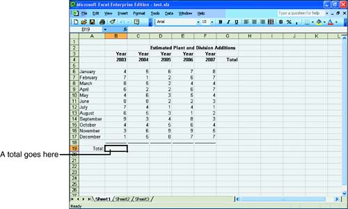
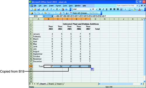
You can combine any and all the operators in a formula. When combining operators, Excel follows the traditional computer (and algebraic) operator-hierarchy model. Therefore, Excel first computes exponentiation if you raise any value to another power. Excel then calculates all multiplication and division in a left-to-right order (the first one to appear computes first) before addition and subtraction (also in left-to-right order). The following formula returns a result of 14 because Excel first calculates the exponentiation of 2 raised to the third power, and then Excel divides the answer (8) by 4, multiplies the result (2) by 2, and finally subtracts the result (4) from 18. Even though the subtraction appears first, the operator hierarchy forces the subtraction to wait until last to compute. =18 - 2 ^ 3 / 4 * 2 If you want to override the operator hierarchy, put parentheses around the parts you want Excel to compute first. The following formula returns a different result from the previous one, for example, despite the same values and operators used: =(18 - 2) ^ 3 / 4 * 2 Instead of 14, this formula returns 2,048! The subtraction produces 16, which is then raised to the third power (producing 4,096) before dividing by 4 and multiplying the result by 2 to get 2,048. Using Range Names in FormulasThe true power of Excel shows when you use cell references and range names in formulas. You learned in an earlier section, "Working with Worksheet Ranges," how to name your worksheet ranges. Instead of referring to the range F2:G14, you can name that range MonthlySales and then refer to MonthlySales in your formulas by name . All the following are valid formulas. Cell references or range names appear throughout the formulas. =(SalesTotals)/NumOfSales =C4 * 2 - (Rate * .08) =7 + LE51 - (Gross - Net) When you enter formulas that contain range references, you can either type the full reference or point to the cell reference. If you want to include a complete named range in a formula (formulas can work on complete ranges, as you see later this hour ), select the entire range and Excel inserts the range name in your formula. Often, finding and pointing to a value is easier than locating the reference and entering it exactly. If, for example, you are entering a formula, when you get to the place in the formula that requires a cell reference, don't type the cell reference; instead, point and click on the cell you want to use in the formula, and Excel adds that cell reference to your formula. If you enter a formula such as =7 + , instead of typing a cell reference of LE51 , you can point to that cell and press Enter or type another operator to continue the formula. Immediately after typing the cell reference for you, Excel returns your cell pointer to the formula (or to the formula bar if you are entering the formula there) so that you can complete it. After you assign a name to a range, you don't have to remember that range's reference when you use it in formulas. Suppose that you are creating a large worksheet that spans many screens. If you assign names to cells when you create them ” especially to cells that you know you will refer to later during the worksheet's development ”entering formulas that use that name is easier. Instead of locating that cell to find its address, you need only to type the name when entering a formula that uses that cell. Relative Versus Absolute Cell ReferencingWhen you copy formulas that contain cell references, Excel updates the cell references so that they cite relative references . For example, suppose that you enter this formula in cell A1: =A2 + A3 This formula contains two references. The references are relative because the references A2 and A3 change if you copy the formula elsewhere. If you copy the formula to cell B5, for example, B5 holds this: =B6 + B7 The original relative references update to reflect the formula's copied location. Of course, A1 still holds its original contents, but the copied cell at B5 holds the same formula referencing B5 rather than A1. An absolute reference is a reference that does not change if you copy the formula. A dollar sign ($) always precedes an absolute reference. The reference $B$5 is an absolute reference. If you want to sum two columns of data (A1 with B1, A2 with B2, and so on) and then multiply each sum by some constant number, for example, the constant number can be a cell referred to as an absolute reference. That formula might resemble this: =(A1 + B1) * $J $J$1 is an absolute reference , but A1 and B1 are relative. If you copy the formula down one row, the formula changes to this: =(A2 + B2) * $J Notice that the first two cells changed because when you originally entered them, they were relative cell references. You told Excel, by placing dollar signs in front of the absolute cell reference's row and column references, not to change that reference when you copy the formula elsewhere. $B5 is a partial absolute cell reference. If you copy a formula with $B5 inside the computation, the $B keeps the B column intact, but the fifth row updates to the row location of the target cell. If you type the following formula in cell A1: =2 * $B5 and then copy the formula to cell F6, cell F6 holds this formula: =2 * $B10 You copied the formula to a cell five rows and five columns over in the worksheet. Excel did not update the column name, B , because you told Excel to keep that column name absolute. (It is always B no matter where you copy the formula.) Excel added 5 to the row number, however, because the row number was relative and open to change whenever you copied the formula. The dollar sign keeps the row B absolute no matter where you copy the formula, but the relative row number can change as you copy the formula. The bottom line is this: Most of the time, you use relative referencing. If you insert or delete rows, columns, or cells, your formulas remain accurate because the cells that they reference change as your worksheet changes. Copying FormulasExcel offers several shortcut tools that make copying cells from one location to another simple. Consider the worksheet in Figure 7.5. The bottom row needs to hold formulas that total each of the projected year's 12-month values. Figure 7.5. A total row is needed for the project's yearly values. How do you enter the total for column B in cell B19? You can type the following formula in cell B19: =B6+B7+B8+B9+B10+B11+B12+B13+B14+B15+B16+B17 There are better ways to total a column of numbers , but for now this way will suffice. As you enter formulas, Excel color -codes cells that you refer to as you type the formula. Therefore, if you create Figure 7.5's worksheet and start typing =B6+B7+ into the total area, Excel colors each cell starting with B6, as well as that cell reference in the formula, a unique color. By color-coding the cells to match the formula references, you can more easily spot mistakes in long formulas. After you type the formula in B19, you then can type the following formula in cell C19: =C6+C7+C8+C9+C10+C11+C12+C13+C14+C15+C16+C17 You then can type the values in the remaining total cells. Instead of doing all that typing, however, copy cell B19 to cell C19. Hold Ctrl while you drag the cell edge of B19 to C19. When you release the mouse, cell C19 properly totals column C! Press Ctrl and copy C19 to D19 through F19 to place the totals in all the total cells. The totals are accurate, as Figure 7.6 shows. Figure 7.6. Relative references make totaling these columns simple. After you drag one or more cells to fill data in other cells, Excel displays the AutoFill Options button at the right of the fill that you can click to specify how you want the new cells to be formatted (the same as the original cell without bringing the original cell's format to the new ones). Generally, the default fill method works well and you'll often never click the AutoFill Options button to change the way Excel completed your cells. |
EAN: 2147483647
Pages: 272