Experiment and Results

---

We performed two different experiments, one each for two different approaches. In this section, we describe the results of both of our experiments.

Experiment 1: Connectionist Model

Based on the design considerations described in the previous section, we conducted three different sub-experiments varying the structural design and noise parameters in a two-layer network. Table 2 and Table 3 illustrate the results of different structural designs for our three sub-experiments for network training on 30 cases and testing the trained network on 10 unseen cases, respectively. The first two sub-experiments represent the hidden number of nodes of 7 and 4 in a two-layer network. The numbers 7 and 4 were chosen to represent (2n+1) and (n+1) heuristic where n is the number of input nodes. No difference in prediction accuracy and RMS during the learning phase was noticed for first two sub-experiments. Since 4 node network represents a smaller network that would converge quickly, in our third experiment, we experimented with adding random input and weight noise (values shown in Table 2) during the training phase of the network.

Table 2: Performance of three different structural designs during the training phase

Number of Hidden Nodes	Input Noise	Weight Noise	RMS Error
7	0	0	0.213
4	0	0	0.213
4	0.08	0.01	0.234

Table 3: Performance of three different networks during the test phase

Number of Hidden Nodes	Input Noise in Trained Net.	Weight Noise in Trained Net.	RMS Error
7	No	No	0.131
4	No	No	0.132
4	Yes	Yes	0.140

The test results of the three trained networks for three sub-experiments on the 10 unseen cases, shown in Table 3, show that the network trained with noise showed higher prediction accuracy and higher RMS error. We plot the training and test results of our third experiment with 4 hidden layers and random input and weight noise in Figures 2 and 3, respectively.

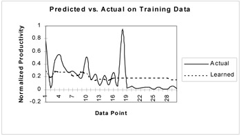
Figure 2: The performance comparison between the actual effort and network learned effort at convergence

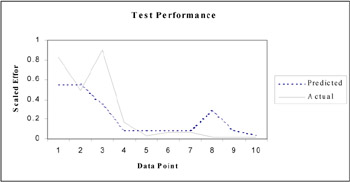
Figure 3: The performance comparison between the actual effort and network predicted effort

Table 4 illustrates the t-test results on difference of means for actual effort and connectionist model learned and predicted effort on training and test data set.

Table 4: Pair-wise comparison (t-test) results for difference in means for actual and predicted software effort

	Training Set (μactual = μpredicted)	Test Set (μactual = μpredicted)
t-value	1.259	0.588
P (T <= t) one tail	0.109	0.285
P (T <= t) two tail	0.218	0.571
*α =0.05

The results in Table 4 indicate that at level of significance of 0.05 the null hypothesis of no difference on means for actual software effort and connectionist model predicted software effort was retained for both training and test data set. The results indicate the utility of using connectionist models for learning and forecasting software effort.

Experiment 2: Evolutionary Model

As described above, our forecasting model during the application of evolutionary learning was represented as:

Software effort = w₁ (development methodology)^w ₂+w₃(tool)^w ₄+w₅ (experience)^w ₆

The set of coefficients, w_i, ∀i ∈ {1, 2, 3, 4, 5, 6} were represented as the population members. The model starts with a number of (equal to the population size=100) random feasible values of w_i. The fitness of each population member is calculated by the value of objective function (Z). Since the objective was to minimize the forecasting error, we modeled our fitness function as, where k₁ was a constant positive number set equal to 10 and actual effort and predicted effort referred to the actual effort in the data set and the predicted effort of a given population member. The objective function was designed to always give positive fitness score for all feasible values of actual and predicted software effort. Crossover and mutation operators are applied in successive generations to explore promising solutions. The crossover rate was set equal to 0.3 and the mutation rate was set equal to 0.1. The feasibility of solutions during the mutation and crossover is maintained using a closed set of operators over the real valued interval of [-1, 1]. For example, if a particular variable say, w_p of a solution vector (population member) X is mutated, the system examines the current domain of w_p dom(w_p) and the new value is taken randomly from this domain. A single-point crossover operator was used to ensure feasibility of the offspring after the crossover. If X and Y are two solution vectors (population members) such that X, Y ∈ F (where F ∈ [-1, 1] is a feasible search space and F ⊆ Rⁿ denotes the search space) then the single-point crossover always yields a feasible solution ∀w_i ∈ [-1, 1].

The CPU run time of the non-linear forecasting model, for population size of 100 and 100 learning generations, over a 400 MHZ pentium II processor was 1.967 seconds. The population converged quickly. Figure 4 illustrates the fitness values of the best member and the average population over different learning generations.

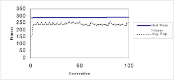
Figure 4: Best member and average population fitness vs. learning generation of the GA run

For the best population member, we plotted the predicted software effort and the actual software effort in the data set. Figure 5 illustrates the result of our plot. The RMS was equal to 0.197, which was lower than that obtained with a similar experiment using the connectionist model. This indicated that the evolutionary model provided a better fit for the training data set.

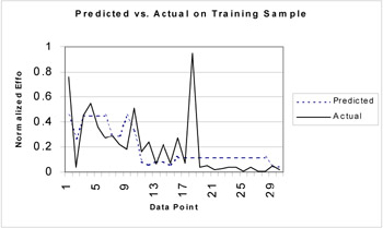
Figure 5: The Performance Comparison between the Actual Effort and the Model Predicted Effort for the Best Fitness Population Member.

Using the best population member we predicted the effort for the test data as well. Figure 6 illustrates the result of our plot. The RMS for the test data set was equal to 0.139 and, when compared to the no-noise case of the connectionist model experiment, the fit was not as good.

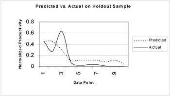
Figure 6: The performance comparison between actual effort and network predicted effort

Table 5 illustrates the result of our t-tests for null hypothesis of no difference in means for actual software effort and predicted software effort using the best population member. For both training data and test data sets, at 0.05 level of significance, the null hypotheses were retained. This provides an evidence that evolutionary model learned and forecasted the software effort correctly.

Table 5: Pair-wise comparison (t-test) results for difference in means for actual and predicted software effort

	Training Set (µactual = µpredicted)	Test Set (µactual = µpredicted)
t-value	1.699	0.743
P (T <= t) one tail	0.438	0.238
P (T <= t) two tail	0.876	0.476
*α =0.05

---