Introductory Concepts and Design Considerations for Non-Linear Connectionist and Evolutionary Models

---

Artificial neural networks (ANNs) and genetic algorithms (GAs) were invented to mimic some of the phenomenon observed in biology. The biological metaphor for ANNs is the human brain and the biological metaphor for GAs is the evolution of a species. An ANN consists of different sets of neurons or nodes and the connections between one set of neurons to the other. Each connection between two nodes in different sets is assigned a weight which shows the strength of the connection. The connections with a positive weight are called excitatory connections and a connection with a negative weight is called an inhibitory connection. The network of neurons and their connections is called the architecture of the ANN. Let A = {N₁, N₂, N₃}, B = { N₄, N₅, N₆}, and C= { N₇} be three sets of nodes for an ANN. The set A is called a set of input nodes, set B is called a hidden set of nodes, and set C is called a set of output nodes. The cardinality of set A is equal to the number of input variables; the cardinality of set C is equal to number of output variables. Each connection can be viewed as a mapping from either an input node to a hidden node or from a hidden node to an output node. The general architecture of three sets of nodes is called a three-layer (of nodes) ANN. Figure 1 illustrates a three-layer ANN. Notice when the property AÇBÇC=F always holds true and the network is called a feed-forward network. The connections in a feed-forward network are in one direction and the connections from A to B and from B to C are onto. The w_ij are the weights that denote the strength of connection from node i to node j.

Figure 1: A three-layer (of nodes) artificial neural network

Information is processed at each node in an ANN. For example, at hidden node N₄ the incoming signal vector (input) from the three nodes in the input set is multiplied by the strength of each connection and is added up. The result is passed through an activation function and the outcome is the activation for the node. If x represents the sum of the product of incoming signal vector and the strength of connection then the activation, using logistic sigmoid activation function, can be represented by,

In the back-propagation algorithm based learning, the strengths of connections are randomly chosen. Based on the initial set of randomly chosen weights, the algorithm tries to minimize the following root mean square error (RMS):

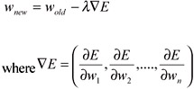
where N is number of patterns in the training set, t_n is the target output of the n^th pattern and o_n is the actual output for n^th pattern. In each subsequent training step, the initial set of random connection weights (strength of connections) is adjusted towards the direction of maximum decrease of E which is scaled by a learning rate lamda. Mathematically, an old weight w_old is updated to its new value w_new using following equation:

One useful property of the sigmoid function is that:

This means that the derivative (gradient) of the sigmoid function can be calculated by applying a simple multiplication and subtraction operator on the function itself. For any neuron n_k, its output is determined by one of the following formulas:

where x_i is the ith input (A is total number of inputs), w_lik is the strength of connection from the ith input node to the kth hidden node, B is number of hidden nodes, w_2ik is the strength of connection from the ith hidden node to the kth output node, and C is number of output nodes. The weights w_10k and w_20k are thresholding weights and x₀ and h₀ are both equal to one. The network is initialized with small random values for the weights, and the back-propagation learning procedure is used to update the weights as the data is iteratively presented to the input-layer neurons. At each iteration, the weights are updated by back-propagating the error as follows:

• ΔWl_ik = ηδ_kx_i and Δw2_ik = η∂_kh_k

where

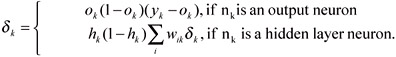
Here, η is the learning rate and y_k is the actual output value.

Genetic algorithms (GAs) use survival of the fittest strategy to learn solution vector for a forecasting model. GAs are a parallel search technique that starts with a set of random potential solutions and uses special search operators (evaluation, selection, crossover, and mutation) to bias the search towards the promising solutions. At any given time, unlike any optimization approach, GA has several promising potential solutions (equal to population size) as opposed to one optimal solution. Each population member in a GA is a potential solution. A population member (P₁) used to obtain solution vector for a forecasting model will consist of a set of all unknown parameters. P₁ can be represented as:

• P₁ = ⟨w₁₄, w₁₅, w₁₆, w₂₄, w₂₅, w₂₆, w₃₁, w₃₅, w₃₆, w₄₇, w₅₇, w₆₇ ⟩

where (w₁₄, w_l5, w_l6, w₂₄, w₂₅, w₂₆, w_3l, w₃₅,w₃₆, w₄₇, w₅₇, w₆₇) ∈ ℜ are unknown parameters in a forecasting model. Any w ∈ P₁ is called a gene (a variable in the forecasting model) of a given population member P_l. A set of several population members is called population Ω. The cardinality of the set of population members Ω (number of population members) is called population size. The cardinality of a population (number of genes) member is called the defining length of the population member ζ. The defining length (number of unknown variables in forecasting model) for population member P₁ is ζ=12. The defining length of all the population members in a given population is constant.

GA starts with a random set of population. An evaluation operator is then applied to evaluate the fitness of each individual. In case of obtaining a forecasting model, the evaluation function is the inverse of forecasting error. A selection operator is then applied to select the population members with higher fitness (lower forecasting error). Under the selection operator, individual population members may be born, allowed to live or die. Several selection operators are reported in literature; the operators are proportionate reproduction, ranking selection, tournament selection, and steady state selection. Among the popular selection operators are ranking and tournament selection. Goldberg and Deb (1991) show that both ranking and tournament selection maintain strong population fitness growth potential under normal conditions. The tournament selection operator, however, requires lower computational overhead. The time complexity of ranking selection is O (nlog n) whereas the time complexity of tournament selection is O(n) where n is the number of population members in a population. In tournament selection two random pair of individuals are selected and the member with the better fitness of the two is admitted to the pool of individuals for further genetic processing. The process is repeated in the way that the population size remains constant and the best individual in the population always survives. For our research, we use the tournament selection operator.

After a selection operator is applied, the new population special operators called crossover and mutation are applied with a certain probability. For applying the crossover operator, the status of each population member is determined. Every population member is assigned a status as a survivor or non-survivor. The number of population members equal to survivor status is approximately equal to population size * (1 - probability of crossover). The number of non-surviving members are approximately equal to population size *probalility of crossover. The non-surviving members in a population are then replaced by applying crossover operators to randomly selected surviving members. Several crossover operators exist; we use one-point crossover in our research.

In one-point crossover, two surviving parents and a crossover point are randomly selected. For each parent, the genes in the right-hand side of the crossover point are flipped to produce two children. Let P₁ and P₂ be two parents and the crossover point be denoted by "|." The two children C₁ and C₂ are produced as follows: (we use the bold font to simplify the understanding).

P₁ = ⟨ w₁₄, w₁₅, w₁₆, w₂₄, w₂₅, w₂₆, | w₃₄, w₃₅, w₃₆, w₄₇, w₅₇, w₆₇ ⟩

P₂ = ⟨ w₁₄, w₁₅, w₁₆, w₂₄, w₂₅, w₂₆, | w₃₄, w₃₅, w₃₆, w₄₇, w₅₇, w₆₇ ⟩

C₁ = ⟨ w₁₄, w₁₅, w₁₆, w₂₄, w₂₅, w₂₆, w₃₄, w₃₅, w₃₆, w₄₇, w₅₇, w₆₇ ⟩

C₂ = ⟨ w₁₄, w₁₅, w₁₆, w₂₄, w₂₅, w₂₆, w₃₄, w₃₅, w₃₆, w₄₇, w₅₇, w₆₇ ⟩

The mutation operator randomly picks a gene in a surviving population member (with the probability equal to probability of mutation) and replaces it with a real random number.

---