Introduction to Bayesian Networks

---

Bayesian networks are classified as graphical, decision-analytical models. Their most remarkable feature is the capability to encode both quantitative and qualitative knowledge. This means, we can rely in this model on statistical data analysis and experience of domain experts as well. Sometimes referred to as causal networks, Bayesian models are constructed as graph models, where nodes are used to encode parameter characteristics (descriptive variables), and directional links between them encode often complex correlations, usually of causal nature.

The network, as a whole, embodies the structure of problem domain, while local interactions between parameters are quantified in the form of conditional probability tables. This representation of modeled phenomenon is in concert with an intuitive approach to its description, which, as is believed, is the basis of the reasoning of human experts. At the same time, Bayesian models are founded on robust statistical methods, despite the fact they are formulated using a non-frequentist definition of probability.

Practical applications of Bayesian networks derive from their analytical and diagnostic capabilities. The constructed model gives us a state-of-knowledge encodement of modeled phenomenon. Information gathered during observation of real phenomenon gives us values of at least some of model parameters—which when stated unambiguously, become facts in the system. In the structure of the Bayesian network this means initialization of the state of nodes to one of possible, predefined values. Propagation of probabilities in network perturbed this way leads to a new equilibrium state, where newly calculated and usually changed probability distributions reflect the fact that new information has been gained. Inspection of new probability distributions makes inference regarding nonobservable variables possible.

It should be mentioned that the number of observed facts could be different, depending on the rate of change of the phenomenon/process, costs of acquiring information or number of variables that cannot be observed directly for different reasons (an example we can bring the prognostic model, where some variables are naturally known post factum).

The Bayesian model reveals in the last case one of its strongest advantages—capability for doing inference when noisy or incomplete data are available.

The propagation of probabilities in Bayesian networks can be of high computational complexity. At the end of the '80s, a significant breakthrough in propagation algorithms was made. Nevertheless, in extreme cases of dense networks or specific topologies, the problem remains NP-hard. Approximate methods of propagation and algorithms tailored to specific structures become of research interests to overcome problem of intractability.

As an elementary toy-problem we describe the following situation:

A bank classifies customers into two categories A and B,

In group A account debiting occurs with 0.2 probability, P(D|A)=0.20,

In group B account debiting occurs with 0.05 probability, P(D|B)=0.05,

15% of all customers belong to group A.

Question: randomly chosen account appears to be debited, what is the probability of its belonging to group A customer?

The problem can be easily solved using Bayes theorem

Table 1: Probability table P(<Customer Category>)

Customer Category
A	B
0.15	0.85
Source: The authors' own research

Table 2: Probability table P(<Customer Category >|<Debit>)

Debit
Customer Category	yes	no
A	0.2	0.8
B	0.05	0.95
Source: The authors' own research

Therefore, we can expect to find a solution using Bayesian networks as well. In fact, the two-node network <Customer Category> linked to <Debit> node models the problem fully.

The network that encodes knowledge of debit statistics in a hypothetical bank is given in Figure 1.

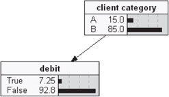
Figure 1: Simple debit model—Uninitialized network

Substituting the actual value of debiting probability, i.e., P(Debit=Yes)=1, after the propagation procedure and reaching equilibrium state of the network, we come to the conclusion that given debiting, the probability of being member of category A customer is 0.414. The solution has been obtained using the Andersen propagation algorithm (Andersen, 1989).

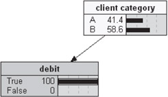
Figure 2: Initialized network after propagation procedure

The given example shows the diagnostic function of the Bayesian model. The network has been used to perform diagnosis of possible causes on the basis of discovered effects. In the situation of reverse state of knowledge, we would be able to infer on effects given states of possible, although not necessarily all, causes.

---