Example Problem: Curve Fitting Specific Heat Data

Let's apply the DataModeling and Polynomial classes to a practical problem ”developing a curve fit expression for the specific heat data of diatomic oxygen . The specific heat data is from the JANAF Thermochemical Tables. ¹ As the name would suggest, this reference provides tables of specific heat, enthalpy, and entropy values as a function of temperature for a wide variety of chemical species. When developing chemical or thermodynamic analysis tools it is often useful to have a mathematical expression for specific heat as a function of temperature. We will obtain such an equation by applying a least squares analysis to the JANAF data. The data we will curve fit is shown in Table 24.1.

If you went through the examples from Chapter 23, you should have already placed the DataModeling.java and Polynomial.java source files in the TechJava\MathLib directory and compiled the files from the package root directory. If you haven't already done that, do it now.

Table 24.1. Diatomic Oxygen-Specific Heat Data

T EMPERATURE, K	S PECIFIC HEAT,
200	29.106
500	31.091
1000	34.870
2000	37.741
3000	39.864
4000	41.421
5000	42.675
6000	44.387

The FifthOrderDemo class is written to curve fit the specific heat data. The code listing is shown next . The first thing the class does is to define x[] and y[] arrays to store the data from Table 24.1. We'll use a fifth-order polynomial expression for the curve fit, so a Polynomial object is created passing the number 5 to the constructor. The leastSquaresFit() method is then called to compute the polynomial coefficients. The resulting polynomial equation is printed to standard output as well as a column of specific heat results.

 import TechJava.MathLib.*; public class FifthOrderDemo {   public static void main(String args[]) {     double x[] = { 200.0, 500.0, 1000.0, 2000.0,                  3000.0, 4000.0, 5000.0, 6000.0 };     //  diatomic oxygen specific heat data     double y[] = { 29.126, 31.091, 34.870, 37.741,                    39.864, 41.421, 42.675, 44.387 };     //  Create a Polynomial object that represents a     //  fifth-order polynomial equation of the form     // y = A5*x^5 + A4*x^4 + A3*x^3 + A2*x^2 + A1*x + A0     Polynomial fifthOrder = new Polynomial(5);     //  Perform a least squares fit on the data.     DataModeling.leastSquaresFit(fifthOrder, x, y);     //  Print out the polynomial equation and some     //  results over a range of temperatures.     double coeff[] = fifthOrder.getCoefficients();     System.out.println("cp = " + coeff[0] + "x^5 + " +           coeff[1] + "x^4 + " + coeff[2] + "x^3 + " +           coeff[3] + "x^2 + " + coeff[4] + "x + " +           coeff[5]);     System.out.println();     double T;     for (int i=0; i<60; ++i) {       T = 100*(i+1);       System.out.println("T = "+T+" cp = "+                           fifthOrder.getValue(T));     }   } } 

Output (removing some decimal places for clarity) ”

[View full width]

 
 [View full width] 
 cp = 9.82625E-18x^5 + -1.80028E-13x^4 + 1.32458E-9x^3 + -5.03019E-6x^2 + 0.01157x + 26.  82537 

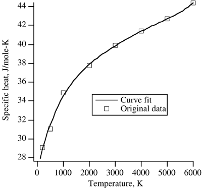
The column of data printed by the FifthOrderDemo class is plotted in Figure 24.1. Also shown on the plot are the original data points. The curve fit equation does an excellent job of reproducing the original data over the entire temperature range. One thing to note, however, is that the curve fit equation would only be reliable for the temperature range over which it was constructed , 200 K to 6000 K. At temperatures below 200 K or above 6000 K, the curve fit equation might give erroneous specific heat values.

Figure 24.1. Least squares curve fit to specific heat data