Solving Improper Integrals

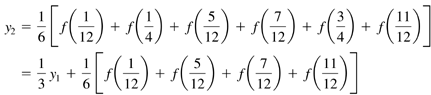
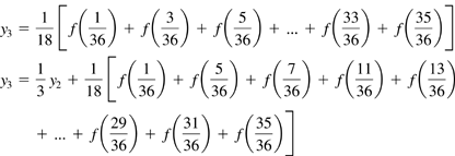
So far in this chapter, we have been exploring methods to solve proper integrals, expressions where the function can be evaluated across the entire integration range and where the limits of integration are finite numbers . Now we turn to the issue of solving improper integrals. If you recall, an improper integral is one that either has an infinite integration limit or one or more singularities in the range of integration.

In some cases, you can turn an improper integral into a proper one and then apply the trapezoidal or Simpson's rule methods. If one or both of the integration limits is positive or negative infinity you can sometimes perform a change of variables to eliminate the infinite limit. For example, the transformation in Eq. (21.15) could be performed on an integral with an upper integration limit of to convert the integral from improper to proper.

Equation 21.15

Eq. (21.15) would require that the function f ( x ) decrease faster than 1/ x ² as x . A similar transformation could be achieved for an integration limit of “ . If both limits are infinity or if one is infinity and the other 0, the best thing to do is to split the integration into pieces and apply the change of variables to one or both.

Now let's look at the case where the integration limits are finite but there is a singularity at one of the limits. We can't use the trapezoidal or Simpson's rule methods because they evaluate the function at the integration limits. Fortunately, there is a family of what are called open formulas that approximate an integral using only points interior to the integration limits. The algorithm we will implement in this chapter is called the midpoint rule and is given by the expression in Eq. (21.16).

Equation 21.16

The midpoint method is second-order accurate similar to the trapezoidal algorithm. It is called a midpoint method because the function evaluations are performed midway between the D x intervals. For example, consider an integration domain between x = 0 and x = 1. A three-point trapezoidal algorithm would evaluate the function at x = 0, x = 1/2, and x = 1. To model that same situation with the midpoint rule, you would evaluate the equation at x = 1/4 and x = 3/4.

Equation 21.17

As with the trapezoid and Simpson's rule methods, a more accurate midpoint solution can be obtained by adding more evaluation points. Once again, if you increase the number of points wisely you can reuse previous evaluations of f ( x ). For example, let's say you start with the two-point midpoint formula shown in Eq. (21.17). If you want to reuse the two function evaluations, the next level in the approximation uses six points (adds four to the two existing points). The six-point midpoint method is defined by the expression in Eq. (21.18).

Equation 21.18

To reuse the function evaluations from the six-point level, the next level in the approximation would add 12 points to the existing six for an 18-point midpoint algorithm.

Equation 21.19

Once again, we can see a pattern developing. Each level in the midpoint approximation adds three times the number of points that were added at the previous level. The value at each new level of approximation is equal to one-third the value at the previous approximation added to the contributions of the additional points added at the current level.

The midpoint method can evaluate an integral with a singularity at one or both of the integration limits, but what happens if a singularity occurs in the middle of the range of integration. The answer is to split the range of integration into two pieces at the singular point. The singularity now occurs at one of the integration limits and the midpoint methodology can be applied.

We will implement the midpoint technique in a method named midpoint() that will be defined in the Integrator class. The method will take the same four input arguments as the trapezoidal() and simpsonsRule() methods. The first argument is a reference to a Function object that is used to evaluate the function being integrated. The second and third arguments are the integration limits. The fourth argument is the convergence tolerance.

After declaring some variables, the method computes a two-point midpoint approximation to the integral equation. It then refines the integral value with successive approximations adding points to the integration domain with each approximation. The first iteration adds four points, the second adds 12 points, the third adds 36 points, and so on. If the integration value converges, the method returns the value.

Here is the midpoint() method source code.

 public static double midpoint(Function function,          double start, double end, double tolerance) {   double dx = end - start;   double value, oldValue, sum, temp;   double scale = 1.0/3.0;   int numPoints, numPairs;   int maxIter = 20;   //  Start with a two-point midpoint   //  evaluation.   value = 0.5*dx*(               function.getValue(start + 0.25*dx) +               function.getValue(end - 0.25*dx) );   //  Refine the solution by adding points to the   //  integration domain. Each iteration adds three   //  times as many points as the previous iteration.   //  When the solution converges, return the result.   for(int i=0; i<maxIter; ++i) {     numPoints = 4*(int)Math.pow(3,i);     numPairs = (numPoints - 2)/2;     temp = 1.0/(3.0*numPoints);     //  Add the two endpoint values to the sum     sum = function.getValue(start + temp*dx) +              function.getValue(end - temp*dx);     //  Add in each pair to the sum     for(int j=0; j<numPairs; ++j) {       sum = sum +         function.getValue(start + (6*j + 5)*temp*dx) +         function.getValue(start + (6*j + 7)*temp*dx);     }     oldValue = value;     value = value/3.0 +             0.5*Math.pow(scale,i+1)*dx*sum;     if ( Math.abs(value-oldValue) <=          tolerance*Math.abs(oldValue) ) {        return value;     }   }   //  Solution did not converge   return 12345.6; } 

Let's test the midpoint() method by applying it to solve two integral equations. Midpoint methods can also be applied to proper integrals, so the first equation to be solved will be the logarithmic integral in Eq. (21.10). The midpoint() method will then be applied to the following improper integral.

Equation 21.20

The integral shown in Eq. (21.20) has a singularity at x = 2, but is convergent and has a value of y = 2. To represent this function, we will define another Function subclass called the SqrtFunction2 class. Its code listing is ”

 package TechJava.MathLib; //  This class represents the function //  y = 1/sqrt(x-2) public class SqrtFunction2 extends Function {    public double getValue(double u) {        return 1.0/Math.sqrt(u-2.0);    } } 

Next we'll create a driver program similar to the ones developed in the previous sections. The code will simply create the proper Function subclass object, call the midpoint() method, and display the result. The class is called TestMidpoint and its source code is ”

 import TechJava.MathLib.*; public class TestMidpoint {   public static void main(String args[]) {     double value;     //  Integrate the function y = x*ln(x) from     //  x=2 to x=4 with an error tolerance of 1.0e-4     LogFunction function = new LogFunction();     value = Integrator.midpoint(                            function,2.0,4.0,1.0e-4);     System.out.println("value = " + value);     //  Integrate the function y = 1/sqrt(x-2) from     //  x=2 to x=3 with an error tolerance of 1.0e-4     SqrtFunction2 function2 = new SqrtFunction2();     value = Integrator.midpoint(                            function2,2.0,3.0,1.0e-4);     System.out.println("value = " + value);   } } 

Output ”

 value = 6.7040209108022335 value = 1.9998044225262488 

The midpoint() method successfully evaluated the integrals to four-decimal place precision. Improper integrals are tougher to compute and generally take significantly more iterations to achieve convergence. In this example, three iterations were required for the proper logarithmic integral but 14 were necessary to converge the improper integral computation.