0991-0995

Previous Table of Contents Next

Page 991

CHAPTER 43

Introducing Oracle Discoverer

IN THIS CHAPTER

• Multidimensional Database Primer 992
• A Semi-Formal Definition of OLAP 997
• Multidimensional Storage Strategies A Star Schema Is Born 999
• Discoverer as a Tool for Data Warehousing 1001
• Discoverer 3.0Features, Functions, and Benefits 1002

Page 992

Welcome to the world of Oracle's Discoverer product. This is one of the most interesting accessories that Oracle offers with their database because it introduces a new database paradigm: the paradigm of multidimensional databases and OLAP processing. OLAP stands for online analytical processing. This is what Discoverer enables you to do.

Before going into the specifics of Discoverer, we will look at what OLAP and multidimensional databases are. You will see how these powerful concepts can add value to your business by allowing you to look at your data in a more intuitive way. It will also become obvious that Discoverer will add value for you by cutting down time on certain programming tasks and on computer resources.

Multidimensional Database Primer

Although the relational model for databases allows great flexibility in defining ways of looking at and processing data, in a business the way that data is processed is often very different from the way that the business analysts would like to look at data. All of us who have any data-
processing experience can recall reports or programs that had to "massage" data into a specific form so a corporate decision-maker could view reports that were meaningful to their overall business.

Consider a point-of-purchase database that does OLTP (online transaction processing) for a nationwide retail sales application. Let us look at the main table Sale and view its column definitions:

 Sale transaction_id customer_id location item unit_price quantity_sold timestamp 

This table will grow in time as sales grow and the system remains online. Customers will return to buy more goods over time and the timestamp, which is the exact date and time of the sale, will begin to trace months and months of sales. Through these months, prices will change, an item will be discounted, and this will further affect the data, which is all comfortably waiting in the sale table to be analyzed .

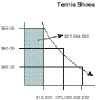
From this simple table designed to store OLTP transactions, we have a hidden wealth of data that business analysts will want to view. For instance, how does price affect the sales of a certain brand of tennis shoes? From a microeconomic viewpoint we might want to plot a demand curve tracing how much price discounting improves the quantity sold for the shoe. After gathering two years of data in our simple table (which is now millions of rows in size ), an analyst might want to map how each distinct price sold. The result of this might look something like Figure 43.1.

Page 993

Figure 43.1.
Plotting the demand function for tennis shoes.

This is all nice and neat, but how do we get the data out of the sales data table and find out how the sales changed for a particular brand of tennis shoes when we changed the price? Using a traditional SQL approach, we might perform the following query to help us deliver the data needed for the above scatter plot:

 select unit_price, sum(quantity_sold) from sale where item = `Tennis Shoes' group by unit_price 

This would give us an output of something like this:

 Price    Quantity .00    432,000 .00    375,000 .95    310,000 

We would then add the computed total revenue for each pricethe price multiplied by the total quantity soldbecause our goal was based on profit (revenue and costs):

 select unit_price, sum(quantity_sold), unit_price * sum(quantity_sold) revenue from sale where item = `Tennis Shoes' group by unit_price 

We would receive the following output:

 Price    Quantity    Revenue .00    432,000    ,440,000 .00    375,000    ,750,000 .95    310,000    ,684,500 

Page 994

Here, we would find out an interesting thing about the elasticity of demand for our tennis shoe, that even though our highest price resulted in a drop in customers, the total revenue brought in at that price exceeded all others. At this point of our OLAP study, the tennis shoe gurus could decide if this revenue was paramount and therefore permanently raise the price to $69.95, or instead, if market penetration was more important and stick with the $45.00 shoe.

What the previous SQL group gy statement is giving us with the third derived column is the area of the bars in our previous bar graph. This area of each bar is the total revenue for the sale of tennis shoes at a given price (see Figure 43.2).

Figure 43.2.
The area under each rectangle represents total revenue.

At this point, the reader might be in awe of the power of SQL and wonder why we are even talking about the multidimensional database. The problem with the preceding model is that in our fictional company we have thousands of different products that need to be analyzed by price or maybe by price and location. If our business analysts want new reports by region so they can alter prices based on the elasticity of demand for a particular region, we would need to perform another SQL statement:

 select location, unit_price, sum(quantity_sold), unit_price * sum(quantity_sold) revenue from sale where item = `Tennis Shoes' group by location, unit_price 

As the executives, business analysts, and buyers all ask for different models and views of the data, we end up doing three inefficient things:

• We tie up human resources. To perform ongoing analysis and reporting on a large OLTP database, we will need many SQL programmers to continually code different requests .

Page 95

• We create a level of disorganization, in that the SQL written one month by one programmer might have satisfied a need of another executive a year earlier. Unless we have a database of all SQL queries, that fact might be missed and we would find ourselves reinventing the wheel by rewriting the same SQL statement. With the high turnover rate of programmers today, this is very common.
• Whenever we ask another question, or even the same question, we tie up a huge number of resources. For Oracle to execute the simple query, we are performing massive sorts in the temporary tablespace and a very long set of reads to the index tablespace ( assuming that item is indexed), and we are typing up the OLTP disks when we get the rowid of the index and read the actual table data (see Figure 43.3).

Figure 43.3. Aggregating data online uses a great deal of resources.

In a more normalized sale database, the item would probably be broken out to its own tablethus compounding the previous processing problems with the use of table joins, which are very costly. If this becomes a common practice, the OLTP system will slow down and sales people all over the world using our system will process sales more slowly, creating longer lines at the stores and interfering with actual business.

This is why OLAP and the multidimensional database are so important to understand: Users need to look at data in ways totally different from the way data appears in a relational database. Because of this, the idea of the multidimensional database has taken flight. It allows users to view data in an endless series of aggregate chunks without the need for generating endless SQL statements.

Multidimensional databases are based on the idea of the data cube. In the previous example, the multidimensional database would manage data in a different way. Each derived column would appear as a separate dimension. The actual data values would define the length or the domain space of each dimension. Let us create a cube to analyze the sale of this tennis shoe over a period of months, for a given location, and at a given price (see Figure 43.4).

Previous Table of Contents Next