12.2 Run-Time Tests
12.2 Run-Time Tests
The goal of run-time tests is to prove that a building block of a piece of software fulfills its specifications. To give the tests sufficient expressive power so as to justify the expense of time and money that goes into them, we must make of them the same demands that we do of scientific experiments: They must be completely documented, and their results must be reproducible and able to be checked by outsiders. It is useful to distinguish between testing individual modules and integrated system tests, though here the boundaries are fluid (see [Dene], Section 16.1).
To achieve this goal in testing modules the test cases must be so constructed that functions can be exhaustively tested to the extent possible, or in other words, that as large a coverage as possible be achieved of the functions being tested. To establish test coverage various metrics can be employed. For example, for C0 coverage what is measured is the portion of instructions of a function or module that are actually run through, or, concretely, which instructions are not run through. There are more powerful measurements than C0 coverage, which take note of the portion of branches that are taken (C1 coverage), or even the portion of paths of a function that are run through. The last of these is a considerably more complex measure then the first two.
In each case the goal must be to achieve as great a coverage as possible with test cases that completely check the behavior of the interface of the software. This covers two aspects that are only loosely connected one with the other: A test driver that runs through all the branches of a function can still leave errors undetected. On the other hand, one can construct cases in which all the properties of a function are tested, even though some branches of the function are not considered. The quality of a test can thus be measured in at least two dimensions.
If to achieve a high degree of test coverage it does not suffice to establish the test cases based simply on knowledge of the specification, which leads to so-called black box tests, it is necessary to take into consideration the details of the implementation in the construction of test cases, a modus operandi that leads to so-called white box tests. An example where we have created test cases for a special branch of a function based only on the specification is the division algorithm on page 51: To test step 5 the special test data on page 62 were specified, which have the effect that the associated code is executed. On the other hand, the necessity of special test data for division by smaller divisors becomes clear only when one considers that this process is passed off to a special part of the function div_l(). What is involved here is an implementation detail that cannot be derived from the algorithm.
In practice, one usually ends up with a mixture of black box and white box methods, which in [Dene] are aptly called gray box tests. However, it can never be expected that one hundred percent coverage is to be achieved, as the following considerations demonstrate: Let us assume that we are generating prime numbers with the Miller-Rabin test with a large number of iterations (50, say) and a corresponding low probability of error ![]() ≈ 10−30 (cf. Section 10.5) and then testing the prime numbers that are found with a further, definitive, primality test. Since the flow of control leads to one or the other branch of the program, depending on the outcome of this second test, we have no practically relevant chance to reach the branch that is followed exclusively after a negative test outcome. However, the probability that the doubtful branch will be executed when the program is actually used is just as irrelevant, so that possibly one can more easily live with doing without this aspect of the test than to alter the code semantically in order to create the test possibility artificially. In practice, there are thus always situations to be expected that require the abandonment of the goal of one hundred percent test coverage, however that is measured.
≈ 10−30 (cf. Section 10.5) and then testing the prime numbers that are found with a further, definitive, primality test. Since the flow of control leads to one or the other branch of the program, depending on the outcome of this second test, we have no practically relevant chance to reach the branch that is followed exclusively after a negative test outcome. However, the probability that the doubtful branch will be executed when the program is actually used is just as irrelevant, so that possibly one can more easily live with doing without this aspect of the test than to alter the code semantically in order to create the test possibility artificially. In practice, there are thus always situations to be expected that require the abandonment of the goal of one hundred percent test coverage, however that is measured.
The testing of the arithmetic functions in the FLINT/C package, which is carried out primarily from a mathematical viewpoint, is quite a challenge. How can we establish whether addition, multiplication, division, or even exponentiation of large numbers produces the correct results? Pocket calculators can generally compute only on an order of magnitude equivalent to that of the standard arithmetic functions of the C compiler, and so both of these are of limited value in testing.
To be sure, one has the option of employing as a test vehicle another arithmetic software package by creating the necessary interface and transformations of the number formats and letting the functions compete against each other. However, there are two strikes against such an approach: First, this is not sporting, and second, one must ask oneself why one should have faith in someone else's implementation, about which one knows considerably less than about one's own product. We shall therefore seek other possibilities for testing and to this end employ mathematical structures and laws that embody sufficient redundancy to be able to recognize computational errors in the software. Discovered errors can then be attacked with the aid of additional test output and modern symbolic debuggers.
We shall therefore follow selectively a black box approach, and in the rest of this chapter we shall hope to work out a serviceable test plan for the run-time tests that follows essentially the actual course of testing that was used on the FLINT/C functions. In this process we had the goal of achieving high C1 coverage, although no measurements in this regard were employed.
The list of properties of the FLINT/C functions to be tested is not especially long, but it is not without substance. In particular, we must convince ourselves of the following:
-
All calculational results are generated correctly over the entire range of definition of all functions.
-
In particular, all input values for which special code sequences are supplied within a function are correctly processed.
-
Overflow and underflow are correctly handled. That is, all arithmetic operations are carried out modulo Nmax + 1.
-
Leading zeros are accepted without influencing the result.
-
Function calls in accumulator mode with identical memory objects as arguments, such as, for example, add_l(n_l, n_l, n_l), return correct results.
-
All divisions by zero are recognized and generate the appropriate error message.
There are many individual test functions necessary for the processing of this list, functions that call the FLINT/C operations to be tested and check their results. The test functions are collected in test modules and themselves individually tested before they are set loose on the FLINT/C functions. For testing the test functions the same criteria and the same means for static analysis are employed as for the FLINT/C functions, and furthermore, the test functions should be run through at least on a spot-check basis with the help of a symbolic debugger in single-step mode in order to check whether they test the right thing. In order to determine whether the test functions truly respond properly to errors, it is helpful deliberately to build errors into the arithmetic functions that lead to false results (and then after the test phase to remove these errors without a trace!).
Since we cannot test every value in the range of definition for CLINT objects, we need, in addition to fixed preset test values, randomly generated input values that are uniformly distributed across the range of definition [0, Nmax]. To this end we use our function rand_l(r_l, bitlen), where we select the number of binary digits to be set in the variable bitlen with the help of the function usrand64_l() modulo (MAX2 + 1) randomly from the interval [0, MAX2]. The first pass at testing must be the functions for generating pseudorandom numbers, which were discussed in Chapter 11, where among other things we employ the chi-squared test described there for testing the statistical quality of the functions usrand64_l() and usrandBBS_l(). Additionally, we must convince ourselves that the functions rand_l() and randBBS_l() properly generate the CLINT number format and return numbers of precisely the predetermined length. This test is also required for all other functions that output CLINT objects. For recognizing erroneous formats of CLINT arguments we have the function vcheck_l(), which is therefore to be placed at the beginning of the sequence of tests.
A further condition for most of the tests is the possibility of determining the equality or inequality and size comparison of integers represented by CLINT objects. We must also test the functions ld_l(), equ_l(), mequ_l(), and cmp_l(). This can be accomplished with the use of both predefined and random numbers, where all cases—equality as well as inequality with the corresponding size relations—are to be tested.
The input of predefined values proceeds optimally, depending on the purpose, by means of the function str2clint_l() or as an unsigned type with the conversion function u2clint_l() or ul2clint_l(). The function xclint2str_l(), complementary to str2clint_l(), is used for the generation of test output. These functions are therefore the next to appear on our list of functions to be tested. For the testing of string functions we exploit their complementarity and check whether executing one function after the other produces the original character string or, for the other order, the output value in CLINT format. We shall return to this principle repeatedly below.
All that now remains to test are the dynamic registers and their control mechanisms from Chapter 9, which in general we would like to include in the test functions. The use of registers as dynamically allocated memory supports us in our efforts to test the FLINT/C functions, where we additionally implement a debug library for the malloc() functions for allocation of memory. A typical function in such a package, of which there are to be found both public-domain and commercial products (cf. [Spul], Chapter 11), is checking for maintenance of the bounds of dynamically allocated memory. With access to the CLINT registers we can keep close tabs on our FLINT/C functions: Every penetration of the border into foreign memory territory will be reported.
A typical mechanism that enables this redirects calls to malloc() to a special test function that receives the memory requests, in turn calls malloc(), and thereby allocates a somewhat greater amount of memory than is actually requested. The block of memory is registered in an internal data structure, and a frame of a few bytes is constructed "right" and "left" of the memory originally requested, which is filled with a redundant pattern such as alternating binary zeros and ones. Then a pointer is returned to the free memory within the frame. A call to free() now in turn goes first to the debug shell of this function. Before the allocated block is released a check is made as to whether the frame has been left unharmed or whether the pattern has been destroyed by overwriting, in which case an appropriate message is generated and the memory is stricken from the registration list. Only then is the function free() actually called. At the end of the application one can check using the internal registration list whether, or which, areas of memory were not released. The orchestrating of the code for rerouting the calls to malloc() and free() to their debug shells is accomplished with macros that are usually defined in #include files.
For the test of the FLINT/C functions the ResTrack package from [Murp] is employed. This enables the detection, in certain cases, of subtle instances of exceeding the vector bounds of CLINT variables, which otherwise might have remained undetected during testing.
We have now completed the basic preparations and consider next the functions for basic calculation (cf. Chapter 4)
add_l(), sub_l(), mul_l(), sqr_l(), div_l(), mod_l(), inc_l(), dec_l(), shl_l(), shr_l(), shift_l(),
including the kernel functions
add(), sub(), mult(), umul(), sqr(),
the mixed arithmetic functions with a USHORT argument
uadd_l(), usub_l(), umul_l(), udiv_l(), umod_l(), mod2_l(),
and finally the functions for modular arithmetic (cf. Chapters 5 and 6)
madd_l(), msub_l(), mmul_l(), msqr_l(),
and the exponentiation function
*mexp*_l().
The calculational rules that we shall employ in testing these functions arise from the group laws of the integers, which have been introduced already in Chapter 5 for the residue class rings ![]() . The applicable rules for the natural numbers are again collected here, where we find an opportunity for testing wherever an equal sign stands between two expressions (see Table 12.1).
. The applicable rules for the natural numbers are again collected here, where we find an opportunity for testing wherever an equal sign stands between two expressions (see Table 12.1).
| Addition | Multiplication | |
|---|---|---|
| Identity | a + 0 = a | a · 1 = a |
| Commutative law | a + b = b + a | a · b = b · a |
| Associative law | (a + b) + c = a + (b + c) | (a · b) · c = a · (b · c) |
Addition and multiplication can be tested one against the other by making use of the definition

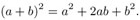
at least for small values of k. Further relations amenable to testing are the distributive law and the first binomial formula:
-
Distributive law :
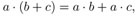
Binomial formula :
The cancellation laws for addition and multiplication provide the following test possibilities for addition and subtraction, as well as for multiplication and division:
![]()
and
![]()
Division with remainder can be tested against multiplication and addition by using the division function to compute, for a dividend a and divisor b, first the quotient q and remainder r. Then multiplication and addition are brought into play to test whether
![]()
For testing modular exponentiation against multiplication for small k we fall back on the definition:

From here we can move on to the exponentiation laws (cf. Chapter 1)

which are likewise a basis for testing exponentiation in relation to multiplication and addition.
In addition to these and other tests based on the rules of arithmetic calculation we make use of special test routines that check the remaining points of our above list, in particular the behavior of the functions on the boundaries of the intervals of definition of CLINT objects or in other special situations, which for certain functions are particularly critical. Some of these tests are contained in the FLINT/C test suite, which is included on the accompanying CD-ROM. The test suite contains the modules listed in Table 12.2.
| Module name | Content of test |
|---|---|
| testrand.c | linear congruences, pseudorandom number generator |
| testbbs.c | Blum-Blum-Shub pseudorandom number generator |
| testreg.c | register management |
| testbas.c | basic functions cpy_l(), ld_l(), equ_l(), mequ_l(), cmp_l(), u2clint_l(), ul2clint_l(), str2clint_l(), xclint2str_l() |
| testadd.c | addition, including inc_l() |
| testsub.c | subtraction, including dec_l() |
| testmul.c | multiplication |
| testkar.c | Karatsuba multiplication |
| testsqr.c | squaring |
| testdiv.c | division with remainder |
| testmadd.c | modular addition |
| testmsub.c | modular subtraction |
| testmmul.c | modular multiplication |
| testmsqr.c | modular squaring |
| testmexp.c | modular exponentiation |
| testset.c | bit access functions |
| testshft.c | shift operations |
| testbool.c | Boolean operations |
| testiroo.c | integer square root |
| testgcd.c | greatest common divisor and least common multiple |
We shall return to the tests of our number-theoretic functions at the end of Part 2, where they are presented as exercises for the especially interested reader (see Chapter 17).
| Team-Fly |
EAN: 2147483647
Pages: 127