23. KPOVs and Data Overview Lean Sigma is different to many traditional Process Improvement initiatives in its reliance on data to make decisions. During Define the major metrics, otherwise known as the Key Process Output Variables[42] (KPOVs) or Big Ys, to measure performance of the process are identified and a ballpark historical value determined. Thenceforth, the equation Y = f(X1,X2,..., Xn) used to identify and narrow down the Xs that drive the Y is completely data driven. [42] Term originates from Dr. Steve Zinkgraf's early work at Allied Signal.
Prior to undertaking that road, it is important to have a basic understanding of data and measures and how to deal with them. There are different ways to categorize data and measures: Continuous versus Attribute Results versus Predictors Efficient versus Effective
The type of data is important because it affects how measures are defined, how to go about collecting data, and which tools to use in analyzing the data, an example is shown in Figure 7.23.1. Figure 7.23.1. Selecting the statistical tool based on the data type. 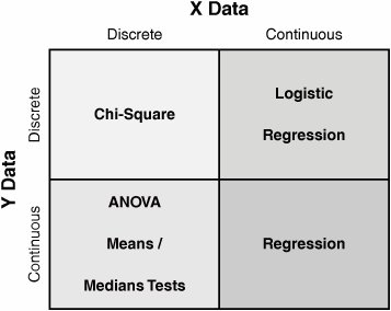
Continuous Measures Continuous measures are those that can be measured on an infinitely divisible scale, such as weight, temperature, height, time, speed, and decibels. They are often called Variable measures. Continuous data is greatly preferred over Attribute type data because it allows the use of more powerful statistical tests and can facilitate decisions being made with much less data (a sample size of 30 works well). Continuous data also allows measurement of performance (i.e., how good is it?) versus conformance (i.e., is it just good or bad?). If the data used in the project is Attribute type, then Belts are strongly encouraged to identify a related Continuous type measure and use that instead. Attribute Measures Any measures that aren't Continuous are known as Attribute or Discrete measures. Despite the lower statistical power, they are generally easier and faster to use than Continuous data and are effective for measuring intangible factors such as Customer Satisfaction or Perception. There are several different types of Attribute data along a spectrum as follows: Binary has just two categories to classify the datafor example, pass/fail, win/lose, or good/bad Categorical or Nominal has multiple categories to classify the data, but there is no order to the categories (there is no greater than or less than involved)for example, U.S. states (Texas, California, and so on), type of product, day of week Rating or Ordinal Scale has multiple categories to classify the data and there is meaningful order to the categoriesfor example, a Likert scale, satisfaction rating 15 Count is a simple count of entitiesfor example, the number of defects or the number of defective items Percentage or Proportion is the count expressed as a percentage or proportion of the totalfor example, the percentage of items scrapped or the proportion of items damaged
As the number of categories increase in Attribute data, the more like Continuous data it becomes. The key failings of Attribute data are the need for a large number of observations to get valid information from any tests performed and also that the data can hide important discrimination. For example, giving Pass or Fail grades in course grading hides the underlying score of each student. Results The Lean Sigma equation Y = f(X1,X2,..., Xn) shows the relationship between the Result (the Y) and the Predictors (the Xs). Results are measures of the process outcomes and are often called "output" factors or KPOVs. Results might be short-term (on-time delivery) or longer-term (Customer satisfaction), but they are typically lagging indicators. Also, because Results are the Ys and are driven by multiple Xs in the process, they are reactive rather than proactive variables. Results tend to be much easier to collect than Predictors and are usually already being measured in the process. Measurement of a Result is typically done against a specification and becomes a Process Capability measure. Predictors Predictors are the "upstream" factors that, if measured, can forecast events "downstream" in the process; for example, an increase in raw-material order lead times might predict an increase in late deliveries. Predictors are the Xs in the equation Y = f(X1,X2,..., Xn) and are often called "input" factors or KPIVs. Predictors are the leading indicators of the process and generally are more difficult to identify and collect. It is unlikely that this data is available historically, so the Team has to set up a measurement system to collect it. Due to the proactive nature of Predictors, they form the basis of the strongest process control measures. Effectiveness There are two categories of metrics used to describe the Big Ys in the process, namely effectiveness and efficiency. Effectiveness is an external measure of the process related to the VOC. An effective process is one that produces the desired results, from the Customer's perspective. To understand effectiveness, the questions to ask relate to How closely are Customers' needs and requirements met? What defects have they received? How satisfied and loyal have they become?
Effectiveness measures include Delivery performance, such as percent on time in full (OTIF) Quality performance, such as problems consumers report with their new product during the first three months of ownership, defects per unit (DPU), or customer percent defective Price, such as relative price index Customer Satisfaction, such as Press Ganey or Gallup Patient Satisfaction scores
Efficiency Efficiency is the second category of metrics used to describe the Big Ys. Efficiency is an internal measure of the process and relates to the level of resources used in the process to achieve the desired result. To understand efficiency, questions to ask relate to how the process performs in the eyes of the business: What is the process cycle time? What is the process yield? How costly is the process at meeting Customer requirements?
Efficiency metrics include Process Lead Time Work content, such as assembly time per unit Process cost, such as labor and materials cost per unit Resources required Cost of poor quality (COPQ), such as Defects per Million Opportunities (DPMO), First Pass Yield, Scrap, Rework, Re-inspect, and Re-audit Percentage of time value-added
Each process and sub-process should have at least two Efficiency requirements established: A ratio of input-to-output value, such as cost per entity processed, process yield A measurement of Cycle Time, such as hours to process an entity
Operational Definitions After a metric has been identified, the work isn't complete. To be a useful metric, a clear, precise description of the metric has to exist. This is critical so that everyone can evaluate and count the same way and there is a common understanding of and agreement on the results. In Transactional processes in particular, Operational Definitions are often the only real way to maintain control and, if poorly defined, are commonly the biggest cause of Measurement System issues. To describe a measure fully, it is useful to create an Operational Definition for it including Who measures (by role, not person's name) What they measure (entities, measurement units) When they measure (timing and frequency) Where they measure (physical location in the process to make measure) How they measure (technique, steps involved) Why they measure (what is the measure used for)
Roadmap The roadmap to identifying, defining, and capturing data is as follows: Step 1. | Identify the measures that translate what is happening in the process into meaningful data. Determine if each measure is a KPOV or KPIV, if it is a measure of Effectiveness or Efficiency, and if it is Continuous or Attribute.
| Step 2. | Create a clear Operational Definition of the characteristic to be measured (who, what, when, where, how, and why).
| Step 3. | Test the Operational Definition with process Stakeholders (all those that affect and are affected by the process) to ensure consistency in understanding. Revise the Operational Definition if necessary. Any metric chosen should be both repeatable and reproducible (see "MSAValidity," "MSAAttribute," and "MSAContinuous" in this chapter).
Belts sometimes believe that there is historical data readily available to complete their project. Historical data can be extremely useful when available; however, it is typically not based on the same operational definitions, hard to use (not stratified the right way, not sortable, and so on,) and generally incomplete. Active data capture is the norm in the vast majority of Lean Sigma projects, so the Team has to create a Data Collection and Sampling plan.
| | | Step 4. | Identify stratification. Before collecting the data, it is important to take time to consider how the Team wants to analyze the data after it is collected. For example, determine which Xs are to be investigated with respect to their effects on the Ys, and so on. To facilitate this, the Xs need to be built into the data collection plan and essentially are means to stratify the data. They might include things such as time, date, person, shift, operation number, Customer, SKU, buyer, machine, subassembly #, defect type, defect location, component and defect impact and criticality, and so on. Be aware though that the number of sub-categories has a big impact on the amount of data required from which to make statistical inferences.
During the Analyze Phase the data is examined and correlated based on these and other Xs. The Xs should come from the Cause & Effect Matrix.
| | | Step 5. | Create a sampling plan.[43] Data collected is only a sample from the process; it never represents every entity to be processed (known as the population). Even if 100% of the data points are collected for the process during a certain period of time, it is still only a sample of the whole population. In fact, this issue drives the use of statistics in the roadmap. Statistics are necessary because there is only a sample taken from the population. The Belt then uses the properties of the sample to draw inferences (predictions, guesses) as to the properties of the population. Clearly there is some guesswork (statistics) involved, but this is a faster, less costly way to gain insight into a process or large population.
[43] For more insight see Statistics for Management and Economics by Keller and Warrack.
The trick is to have the best sample from which to make inferences. Thus the sample needs to be a miniature version of the populationjust like it, only smaller. To achieve this, there are generally two main considerations when samplingsample quality and sample size.
Sample Quality is a measure of how well the sample represents the population and meets the needs of the sampler. Lean Sigma statistical methods generally assume random sampling in which every entity or member of the full population has an equal chance of being selected in the sample. Whichever sampling approach is taken, the Team must strive to
Minimize bias in the sampling procedure. Bias is the difference between the nature of the data in the sample and the true nature of the entire population. A good example of a bias mistake occurred recently for a Belt in a client hospital. The Team chose to track sample medication orders using bright orange paper versus the regular white orders. Given the choice of which to process first, operators always picked orange over white; thus, the timings for the sample were lower than they should have been if the had been truly representative. Avoid "convenience" sampling. Difficult Customers are hard to capture data from but represent a valuable source of information. Minimize "non-response bias." If the likely responders hold different views to the non-responders, then there is a bias. This is common in pre-election surveys when the polls often show a large swing away from the incumbent party because dissatisfied electors tend to take time to air their views to the sampling Team. Minimize data errors and missing data.
It is best to use a standard Sampling Strategy, as listed in Figure 7.23.2.
Figure 7.23.2. Standard Sampling Strategies. 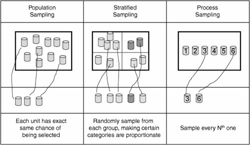
Sample Size is important because, generally, precision in sampling results increases as the Sample Size n increases. Unfortunately, this is not a one-to-one relationship. In fact, mathematically it increases in proportion to  and so doubling sample size doesn't double accuracy. For example, when the sample size increases from 1 to 100, inaccuracy decreases by only 1/10th, and, therefore, it is important to keep sample sizes relatively small. and so doubling sample size doesn't double accuracy. For example, when the sample size increases from 1 to 100, inaccuracy decreases by only 1/10th, and, therefore, it is important to keep sample sizes relatively small.
For Continuous data meaningful Sample Sizes are
For Attribute Data meaningful Sample Sizes are
| | | Step 6. | Based on the Sampling Plan, create a data collection form and tracking system. This comprises the who, what, where, when, and how the data is captured. Some common methods include
Check sheetsData is collected in Attribute form as a series of check marks corresponding to types of defect or similar, see Figure 7.23.3. Figure 7.23.3. An example of a Check sheet. 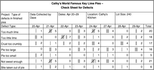 Frequency Plot Check sheetAn extension of the Check sheet in which the defects are recorded directly into a Dot Plot, see Figure 7.23.4. Figure 7.23.4. An example of a Frequency Plot Check sheet. 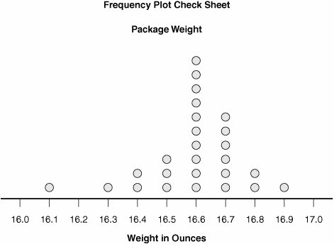 Concentration Diagram Check sheetUsed to mark defects on a physical representation of the product or process, see Figure 7.23.5. The pattern of defects builds to show where the problems occur most often. Figure 7.23.5. An example of a Concentration Diagram.  Data sheetUsed to record continuous data, or a mix of both Continuous and Attribute data. It is best to create the Data sheet directly in a spreadsheet or statistical software in preparation for data analysis, see Figure 7.23.6. Figure 7.23.6. An example of a Data sheet.Operator | Shift | Script | Sales | Time |
|---|
Bob | AM | 1 | 109.57 | 24.07 | Jane | PM | 1 | 173.37 | 26.01 | Jane | PM | 1 | 124.00 | 24.57 | Jane | AM | 1 | 217.38 | 23.70 | Walt | PM | 1 | 154.88 | 27.64 | Jane | AM | 1 | 91.30 | 27.56 | Jane | AM | 1 | 123.99 | 25.16 | Bob | AM | 1 | 138.47 | 25.23 |
Traveler Check sheetUsed to record information about individual items (applications, order forms, products, patients, and so on) as they move through the steps of the process. The easiest way to describe this is to imagine being stapled to the process entity and going along for the ride! A traveler is useful when the process is complex, and an understanding is needed for what happens to each entity as they flow through the process. However, this approach does require additional data preparation steps to bring together all the travelers at the end of data collection. SurveysFor more information see "Customer Surveys" in this chapter.
Whichever data collection format is chosen, it should include data source information, such as Time, Lot Number, Shift, Site, Data Collector's Name, and so on. It is also important to include a Comments section to allow for the recording of any informative conditions. The capture method should always be kept simple and easy-to-read.
A Data Collection Plan Summary sheet is a useful addition to the project, as shown in Figure 7.23.7. The Team then has a complete list of the who, what, where, when, and how for the data collection.
Figure 7.23.7. An example of a Data sheet 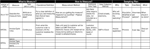
| Step 7. | Create procedures for completing the data collection forms. Any instructions should be visual and understandable by all. It is useful to include pictures of the form, describe what goes in each box and include examples of completed forms. Choose the data collectors carefully and train them on the procedures using the instructions to ensure consistent data collection.
| Step 8. | Test the data collection method. Do a short dry run of the data capture (a few data points) to identify problems and make adjustments. After completion, assess the accuracy, repeatability, and reproducibility of the data collection system (see "MSAValidity," "MSAAttribute," and "MSAContinuous" in this chapter).
| Step 9. | Collect the Data as per the Data Collection Procedure. The Team must follow the Sampling Plan consistently and record any changes in operating conditions not part of the normal or initial operating conditions. Any events out of the ordinary should be immediately written into a logbook. The Belt for the project should check that data collection procedures are followed at all times. When the desired sample size is reached, stop data collection.
| Step 10. | Enter the collected data promptly into a database, such as a spreadsheet or statistical software. Make a backup copy of the electronic file. Keep all the paper copies to be archived as part of the project report.
|
|