K. High Schedule Variation Overview Scheduling, from a process perspective, is effectively a guess as to what the process should be doing at a certain point in time in the future. Interestingly enough, this Problem Category (and the closely related Forecasting equivalent in Section U in this chapter) seems to be one of the first problems requested early in any deployment of Lean Sigma. This is usually due to a misunderstanding of the root cause of the problem. Often (mistakenly), the belief is that if a perfect schedule could be generated, then running the process would be straightforward. In fact, the reality is that it is a more responsive process that creates better scheduling, rather than the other way around. Hence, the initial focus should be on reducing Process Cycle Time and more importantly Process Lead Time to make the durations more predictable and thus be able to generate a better schedule. For more detail see "TimeProcess Lead Time" and "TimeGlobal Process Cycle Time" in Chapter 7, "Tools." In parallel with efforts to make the process more responsive, look at the interaction with downstream Customers to smooth variability in demand (understand causes of cancellations, for example). Finally, after all opportunity has been captured, look at the scheduling approach (usually an algorithm) itself. Examples Industrial. Not a common problem, perhaps delivery scheduling Healthcare. Operating room scheduling, outpatient scheduling Service/Transactional. Delivery scheduling
Measuring Performance The most common way to measure performance of a schedule is to use variance to schedule. Note that the term variance here is not the statistical term variance; it just means the difference between actual and planned. This is measured as follows: Consider the scheduled start time for each scheduled entity to be zero. If an entity actually starts early versus schedule, record a negative offset in time (5 minutes early would read 5 minutes) and conversely a positive offset if it actually starts late. The roll-up would be by the mean and standard deviation of this column of offsets, with a goal of zero mean and minimal variation (standard deviation).
Tool Approach |  | First the variance metric itself needs to be agreed upon by the Champion, Process Owner, and Belt. Next, look at validity of the metrica sound operational definition and consistent measure versus a detailed investigation of Gage R&R will suffice. For more details see "MSAValidity" in Chapter 7. | |  | Take a baseline measure of variance to schedule. This will always be somewhat of a moving target, so pick a point in time and stick to it. For more details see "CapabilityContinuous" in Chapter 7. There might be a need to stratify the metric by entity type (e.g., variance by procedure type in a surgery). This is not absolutely necessary at this stage, but will need to be done later anyway, so it's usually best to just go ahead and stratify as well as get a total variance across all entity types. |
The vast majority of improvements to scheduling doesn't come from improving the scheduling processes directly, but by eliminating noise from the operations process itself (i.e., the process that is being scheduled). Eliminating noise in the operations process will dramatically improve our ability to schedule accurately, but after the noise in the process is reduced, there might still be genuine reasons to look at scheduling. In effect, we have simplified the problem into two phases as follows: Improve the operations process. Improve the scheduling process.
For Phase 1, there are a few Problem Categories to resolve in order of importance: |  | The tools approach that enables a shortening of Process Lead Time will help make the process duration more predictable. For more details see "TimeGlobal Process Lead Time" in Chapter 7. This is usually a good candidate for a kaizen[6] event in that typically no science is required; it's really just a case of removing NVA activity and streamlining the process. Go to Section G in this chapter and then return to this point. | |  | Interestingly, the majority of variability in process duration doesn't appear in the VA work done on the entity, but rather in the NVA work done in changeover between entities or entity types. Again, this is good candidate for a kaizen. Go to Section O in this chapter to resolve this and then return to this point. |
[6] Kaizen is a 25 day rapid change event focused on streamlining a process by removing NVA activities and improving flow. The event gathers a team of the right people together, those that live and breathe the process every day, along with an objective facilitator. The team is charged with understanding and resolving the process issues during the event itself using Lean tools and techniques.
During the work in reducing the Process Lead Time and the Changeover Times, there will have been baseline data captured around the performance of the process. Examine this data to ensure that the following don't apply (if they do, it might be necessary to resolve them first): |  | On average, the process does not have enough capacity (the Cycle Time is longer than its Takt Time). For more details see "TimeTakt Time" in Chapter 7. The process will never generate enough entities to meet demand. Go to Section B in this chapter to resolve this and then return to this point. | |  | On average, the process has enough capacity (the Cycle Time is shorter than the Takt Time), but the process fails intermittently. On average, the process can meet demand (including peaks), but the process is not robust enough to do so on a continuous basis. Go to Section F in this chapter to resolve this and then return to this point. |
After the Phase 1 work, the operations process should be a lot more consistent and thus predictable. It is often the case that the scheduling problem has been resolved at this point. To that end, it is important to revisit Capability at this point. |  | Take a measure of variance to schedule. If stratification was used in the baseline performance, use it again here. | |  | From the Capability data, judge whether the variance to schedule meets business requirements. If it does, proceed to the Control tools in Chapter 5. If not, continue to Phase 2 (next). |
For Phase 2, the Team needs to look to the processes that bring bookings to the schedule and what drives variability in the durations of those entities. This will come from examination of external factors as well as internal (operations) factors. | 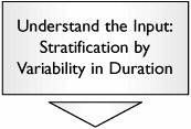 | Some entity types have consistent process duration (and hence are easy to schedule precisely), whereas others are highly variable (and thus difficult to schedule precisely). It is beneficial to consider each separately. List all the entity types and for each collect data for their duration for 25 to 100 data points. Calculate the standard deviation for each. Sort the types by standard deviation. If fewer than 25 data points are available, consider using the range instead of the standard deviation. | | 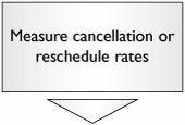 | Cancellations and rescheduling often drive significant scheduling problems. For each of the stratified entity types, gather cancellation and rebooking rates (simply as number canceled/rebooked versus number booked) for a period of one month or more. |
These two steps will allow the Team to segregate the entity types into three populations: | 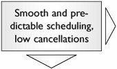 | Leave as is. | | 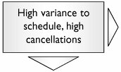 | Seek to understand the cancellation process; look at the process of how the Customer books (from their perspective) and what impacts them showing up. Go to Section C in this chapter to identify Xs that drive cancellation and rebooking, and determine how to reduce them or get more advanced warning. Return here to continue down this roadmap. | |  | The factors driving variance to schedule are not cancellations and rebooking. The scheduling algorithm used is not representative of the Xs that drive variation in duration of the operations process. Continue in this roadmap. |
The roadmap from this point forward is one of the most unusual in Lean Sigma in that the Measure/Analyze will be done on the operations process to identify the Xs that drive the duration, and the Improve/Control will be done on the scheduling process to utilize the identified Xs to better approximate the duration during scheduling. | 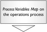 | This tool will identify all input variables (Xs) that drive duration in the operations process (not the scheduling process). It might be worthwhile to also use a Fishbone Diagram at this point to ensure no Xs are overlooked. | | 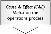 | The Xs generated by the Process Variable Map are transferred directly into the C&E Matrix. The Team uses its existing knowledge of the process through the matrix to eliminate the Xs that don't affect duration. If the process has many steps, consider a three-phase C&E Matrix as follows: Phase 1 List the process steps (not the Xs) as the items to be prioritized in the C&E Matrix. Reduce the number of steps based on the effect of the steps as a whole on duration. Phase 2 For the reduced number of steps, enter the Xs for only those steps into a second C&E Matrix and use this matrix to reduce the Xs to a manageable number. Phase 3 Make a quick check on Xs from the steps eliminated in Phase 1 to ensure that no obviously vital Xs have been eliminated.
| | 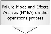 | The reduced set of Xs from the C&E Matrix are entered into the Process Failure Mode and Effects Analysis. This tool will narrow them down further, along with the useful byproduct of generating a set of action items to eliminate or reduce variation in process duration. | |  | The reduced set of Xs from the FMEA is carried over into this array of tools with the Y being operations process duration. Statistical tools applied to actual process data will help answer the questions: Which Xs (probably) affect the duration? Which Xs (probably) don't affect the duration? How much variation in the duration is explained by the Xs investigated?
The word probably is used because this is statistics and hence there is a degree of confidence associated with every inference made. This tool will narrow the Xs down to the few key Xs that (probably) drive most of the variation in duration. In effect, a simple model can be generated that derives the duration based on the levels of the Xs for a particular entity. |
When the Multi-Vari Study is complete, there should be a reasonably sound understanding of which Xs drive the duration and how. There will inevitably be some unexplained variation (noise) too. Often at this point the desire is to optimize to the nth degree, but generally, due to the noise in any operations process, a good approximation is as good as it gets. Sometimes it is possible to take this roadmap further by looking at Designed Experiments, but in general there should be enough understanding at this juncture to resolve the lion's share of the problem. |  | In order to get a better schedule, the scheduling processes and procedures need to be updated to collect the key X data (identified in the Multi-Vari) for all entities. For instance, in the surgery scheduling example, if Body Mass Index (BMI) is identified as a key driver for surgery duration, it needs to be asked for, or calculated, during the scheduling process. | |  | The scheduling algorithm needs to be changed to reflect the new understanding of which Xs drive duration and how. There is a vast array of scheduling software on the market, so there is no single answer here. Quite often, businesses resort to manipulating the schedule by hand or use look-up tables for an interim period until a software update is made. |
After the improvements have been made to the scheduling system, move to the Control tools in Chapter 5. |