3.6 Appendix

3.6.1 Proofs for Section 3.3.1

Proof of Theorem 3.1

Denote and . We have the following differential (at Y ):

Equation 3.231

The differential of the form II group -blind detector,

Equation 3.232

is then given by

Equation 3.233

It then follows from Lemma 2.6 that is asymptotically Gaussian. To find C _w , notice that u ₁ range ( U _s ). Hence, by Proposition 2.6, we have

Equation 3.234

with

Equation 3.235

Equation 3.236

Therefore, the asymptotic covariance of is given by

Equation 3.237

It is easily verified that QY u ₁ = . Using this and the facts that w ₁ = Y u ₁ and QU _n = U _n , by substituting (3.234) into (3.237), we obtain (3.61).

Proof of Corollary 3.1

In this appendix e _k denotes the k th unit vector in and denotes the k th unit vector in . Denote and . Denote further that and . Note that ( Ys _k ) is the linear MMSE detector for the k th user , given by

Equation 3.238

Denote

Equation 3.239

Equation 3.240

Equation 3.241

Equation 3.242

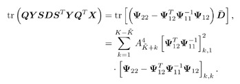
First we compute the term tr ( C _w C _r ). Using (3.61) and the facts that , we have

Equation 3.243

The term ( ) in (3.243) can be computed as

Equation 3.244

Using the fact that , the term tr ( QYQ ^T X ) in (3.243) is given by

Equation 3.245

To compute the second term in (3.243), first note that . We have

Equation 3.246

where the first equality follows from the fact that QY = . Moreover,

Equation 3.247

where we used the fact that YXY = Y . In (3.246) is given by

Equation 3.248

Equation 3.249

Substituting (3.247) and (3.249) into (3.246) we obtain the second term in (3.243):

Equation 3.250

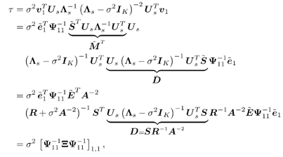
Finally, we compute t in the last term in (3.243). By definition,

Equation 3.251

where

Equation 3.252

Equation 3.253

Equation 3.254

with . Substituting (3.244), (3.245), (3.250), and (3.251) into (3.243), we have

Equation 3.255

Moreover, we have

Equation 3.256

Next we compute w ₁ ² . Since

Equation 3.257

Equation 3.258

we have

Equation 3.259

By (3.255) “(3.259) we obtain the corollary.

SINR Calculation for Example 2

Substituting (2.338) “(2.340) and A ² = A ² I _K into (3.66) “(3.68), we have

Equation 3.260

Equation 3.261

Equation 3.262

Equation 3.263

Equation 3.264

where , , denotes an all-1 -vector, and denotes an all-1 ( )-vector. After some manipulations, we obtain the following expressions:

Equation 3.265

Equation 3.266

Equation 3.267

Equation 3.268

Equation 3.269

Equation 3.270

Substituting (3.265) “(3.270) into (3.69) “(3.72), and letting

Equation 3.271

Equation 3.272

Equation 3.273

Equation 3.274

Equation 3.275

we obtain (3.82).

3.6.2 Proofs for Section 3.3.2

Proof of Theorem 3.2

We prove this theorem for the case of a linear group-blind hybrid detector (i.e., ). The proof for a linear group-blind MMSE detector is essentially the same.

Denote e _k as the k th unit vector in . Let Q ₁ be an orthogonal transformation such that

Equation 3.276

For any , denote . The corresponding projection matrix in the Q ₁ - rotated coordinate system is

Equation 3.277

Equation 3.278

Equation 3.279

Denote

Equation 3.280

Equation 3.281

where the dimension of is (N “ ) x (N “ ). Hence

Equation 3.282

Let the eigendecomposition of be ^[1]

^[1] The eigenvalues are unchanged by similarity transformations.

Equation 3.283

Define another orthogonal transformation,

Equation 3.284

For any , denote . In what follows, we compute the asymptotic covariance matrix of the detector in the Q ₁ Q ₂ -rotated coordinate system. In this new coordinate system, we have

Equation 3.285

Equation 3.286

Equation 3.287

Equation 3.288

Furthermore, after rotation, has the form

Equation 3.289

for some . After some manipulations, the form I group-blind hybrid detector in the new coordinate system has the form

Equation 3.290

where E _s consists of the first columns of (i.e., = [ E _s E _n ]). Let the estimated autocorrelation matrix in the rotated coordinate system be

Equation 3.291

Let the corresponding eigendecomposition of be

Equation 3.292

Then the estimated detector in the same coordinate system is given by

Note that in such a rotated coordinate system, estimation error occurs only in the first elements of . Denote

Equation 3.293

Equation 3.294

Hence is a function of and its differential at (i.e., and is given by

Equation 3.295

By Lemma 2.6, is then asymptotically Gaussian with a covariance matrix given by

Equation 3.296

We next compute the three terms T ₁ , T ₂ , and T ₃ in (3.296).

We first compute T ₁ . Denote z _k and x _k as the subvectors of containing, respectively, the first N “ and the last elements of (i.e., ) for k = + 1, . . . , K . Let . It is clear that range ( U _s ), and therefore range ( ). Expressed in the rotated coordinate system, we have range ( E _s ). We can therefore apply Proposition 2.6 to T ₁ to obtain

Equation 3.297

with

Equation 3.298

Equation 3.299

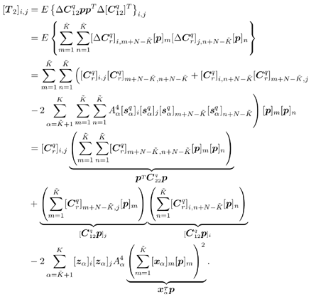
The term T ₂ can be computed following a similar derivation as in the proof of Theorem 1 for the DMI blind detector. Specifically, we have, similar to (2.302),

Equation 3.300

Writing (3.300) in matrix form, we have

Equation 3.301

with

Equation 3.302

Hence the second term in (3.296) is

Equation 3.303

where we have used the fact that , and the definition in (3.293).

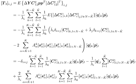
Finally, we calculate T ₃ . Denote . By following the same derivation leading to (2.313), we get for i K “ ,

Equation 3.304

As before, we only have to consider [ T ₃ ] _i,j for i,j K “ or i,j > K “ . However, all terms corresponding to i,j > K “ will be nulled out because of the multiplication of Y on T ₃ . Using Lemma 2.5, we then get (for i,j K “ )

Equation 3.305

Writing this in matrix form, we have

Equation 3.306

Equation 3.307

Hence the third term in (3.296) is given by

Equation 3.308

Substituting (3.297), (3.303), and (3.308) into (3.296), we obtain

Equation 3.309

where D ₁ and D ₂ are given, respectively, by (3.299) and (3.302), and t is given by (3.298). Theorem 3 is now easily obtained by transforming (3.309) back to the original coordinate system according to the following mappings: , , , and .