Feeling a Little Congested?
| When a device, such as a switch or a router, receives traffic faster than it can be transmitted, the device attempts to buffer (that is, store) the extra traffic until bandwidth becomes available. This buffering process is called queuing or congestion management. Routers contain both a hardware queue and a software queue. The router automatically determines the size of the hardware queue, and the first packet to go into the hardware queue is the first packet to exit it. However, after the hardware queue fills to capacity, the software queue accommodates additional packets, and you can use queuing mechanisms to influence the order in which various traffic types are emptied from the software queue, as shown in Figure 6-8. Figure 6-8. Software Queue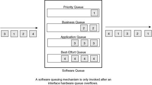 Congestion occurs not just in the WAN but also in the LAN. Mismatched interface speeds, for example, could result in congestion on a high-speed LAN. Aggregation points in the network can also result in congestion. For example, perhaps multiple workstations connect to a switch at FastEthernet speeds (that is, 100 Mbps), and these workstations simultaneously transmit to a server also connected to the same switch via FastEthernet. Such a scenario can result in traffic backing up in a queue. Cisco routers and switches support multiple queuing mechanisms. Before delving into modern queuing methods, such as Low Latency Queuing (LLQ), first consider a few of the Cisco legacy queuing mechanisms. First-In, First-Out (FIFO) QueuingFIFO queuing does not truly perform any QoS operations. As FIFO's name suggests, the first packet to come into the queue is the first packet sent out of the queue, as shown in Figure 6-9. Routers use FIFO queuing in their hardware queue. FIFO in the software queue works just like FIFO in the hardware queue (that is, no packet manipulation occurs). Interfaces running at speeds greater than 2.048 Mbps use FIFO queuing by default. Figure 6-9. First-In, First-Out (FIFO) Queuing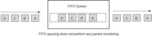 While FIFO is widely supported on all IOS platforms, it can starve out traffic by allowing bandwidth-hungry flows to take an unfair share of the bandwidth. For example, if FTP file transfer packets and voice packets simultaneously reside in a queue, the bandwidth-hungry nature of FTP could starve out the voice packets, causing noticeable gaps in the voice. Weighted Fair Queuing (WFQ)WFQ is enabled by default on slow-speed interfaces (that is, 2.048 Mbps and slower). WFQ allocates a queue for each flow, for as many as 256 flows by default. WFQ uses IP Precedence values to provide a weighting to Fair Queuing (FQ). When emptying the queues, FQ does byte-by-byte scheduling. Specifically, FQ looks 1 byte deep into each queue to determine whether an entire packet can be sent. FQ then looks another byte deep into the queue to determine whether an entire packet can be sent. As a result, smaller traffic flows and smaller packet sizes have priority over bandwidth-hungry flows with large packets. In the following example, three flows simultaneously arrive at a queue. Flow A has three packets, which are 128 bytes each. Flow B has a single 96-byte packet. Flow C has a single 70-byte packet. After 70 byte-by-byte rounds, FQ can transmit the packet from Flow C. After an additional 26 rounds, FQ can transmit the packet from Flow B. After an additional 32 rounds, FQ can transmit the first packet from Flow A. Another 128 rounds are required to send the second packet from Flow A. Finally, after a grand total of 384 rounds, the third packet from Flow A is transmitted, as shown in Figure 6-10. Figure 6-10. Fair Queuing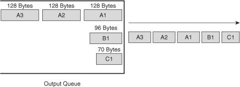 With WFQ, packets' IP Precedence values influence how the packets are emptied from a queue. Consider the previous scenario with the addition of IP Precedence markings. In this scenario, Flow A's packets are marked with an IP Precedence of 5, while Flow B and Flow C have default IP Precedence markings of 0. The order of packet servicing with WFQ is based on sequence numbers, where packets with the lowest sequence numbers are transmitted first. Sequence numbers remind me of my barbershop. My barbershop has a sign reading, "Please take a number." I can pull a number from a dispenser, and when they call my number, it's my turn to get my hair cut. Sequence numbers work the same way. Each packet in the queue is assigned a sequence number, and lower numbers get to go first, just like customers in my barbershop. The sequence number is the weight of the packet multiplied by the number of byte-by-byte rounds that must be completed to service the packet, just as in the FQ example. The Cisco IOS calculates a packet's weight differently depending on the router's IOS version. In older versions of the Cisco IOS (prior to IOS 12.0(5)T), the formula for weight was
In more recent versions of the IOS, the formula for weight is
Using the pre-IOS 12.0(5)T formula (to make the math simpler), the sequence numbers for the previously described packets are
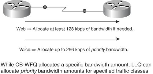
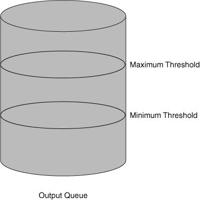
Therefore, after applying the weight, WFQ empties packets from the queue in the following order: A1 A2 A3 C1 B1, as shown in Figure 6-11. Compare that WFQ packet order with the FQ packet order of C1 B1 A1 A2 A3. Figure 6-11. Weighted Fair Queuing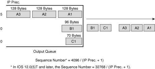 Priority Queuing (PQ)Unlike FIFO and WFQ, priority queuing allows you to specify high-priority traffic and instruct the router to send that traffic first. Priority queuing places traffic into one of four queues (that is, High, Medium, Normal, and Low). Each queue receives a different level of priority, and higher-priority queues must be completely emptied before any packets are emptied from lower-priority queues, as shown in Figure 6-12. This behavior can starve out lower-priority traffic. Figure 6-12. Priority Queuing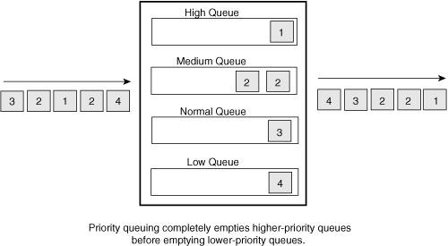 To better understand priority queuing, consider an analogy. Imagine you want to purchase portable MP3 players for all your friends and family this holiday season. For illustrative purposes only, assume an MP3 player costs $1 at Wal-Mart, $10 at K-Mart, $100 at Target, and $1000 at Circuit City. From where do you buy your first MP3 player? Probably Wal-Mart. From where do you buy your second MP3 player? Do you want to spread the wealth around, and buy the second MP3 player from K-Mart? Based on the price difference, you're going to buy your second, third, and fourth MP3 players from Wal-Mart, too. In fact, you'll keep buying MP3 players from Wal-Mart until Wal-Mart is out of stock. Once Wal-Mart is out of MP3 players, and you still need to buy more, where do you go? Based on the prices, you'll probably buy your next MP3 player from K-Mart. Let's jump to the end of the story and ask, "When would you ever buy an MP3 player from Circuit City?" Based on our very fictitious prices, you would only buy an MP3 player from Circuit City when Wal-Mart, K-Mart, and Target were all out of stock. The same logic applies to priority queuing. As long as the High queue contains packets, no packets from the Medium, Normal, or Low queues are transmitted. Packets from the Medium queue can only be sent when the High queue is completely empty, and the only time packets are transmitted from the Low queue is when the High, Medium, and Normal queues are all empty. While priority queuing can offer special traffic, such as voice, high-priority treatment, priority queuing's strict approach tends to starve out lower-priority traffic. Class-Based Weighted Fair Queuing (CB-WFQ)The WFQ mechanism makes sure no traffic is starved out, unlike PQ. However, neither WFQ nor PQ makes a specific amount of bandwidth available for defined traffic types. You can, however, specify a minimum amount of bandwidth to make available for various traffic types using the CB-WFQ mechanism. CB-WFQ can specify bandwidth amounts for up to 64 classes of traffic. Traffic for each class goes into a separate queue. Therefore, one queue (for example, for CITRIX traffic) might be overflowing, while other queues are still accepting packets. Therefore, CB-WFQ gives you the benefit of specifying an amount of bandwidth to give to different traffic classes, something you cannot do with WFQ or PQ. Also, CB-WFQ does not starve out lower-priority traffic as PQ does. The only major downside to CB-WFQ is its lack of a priority queuing mechanism. PQ can give priority treatment to specific traffic, such as voice traffic, while CB-WFQ cannot. A slight modification to CB-WFQ called LLQ fixes this issue. Low Latency Queuing (LLQ)LLQ bears a strong resemblance to CB-WFQ. In fact, LLQ is almost identical in its configuration to CB-WFQ. However, LLQ can instruct one or more traffic classes to direct traffic into a priority queue. Realize that when you place packets in a priority queue, you are not only allocating a bandwidth amount for that traffic, but you are also policing (that is, limiting the available bandwidth) for that traffic. The policing option is necessary to prevent high-priority traffic from starving out lower-priority traffic, as PQ might do. Note that if you tell multiple traffic classes to give priority treatment to their packets, all priority packets go into the same queue. Therefore, priority traffic could suffer from having too many priority classes. Also, be aware that packets queued in the priority queue cannot be fragmented, which is a consideration for slower-speed links (that is, link speeds less than 768 kbps). LLQ, based on all of these benefits, is the Cisco preferred queuing method for latency-sensitive traffic, such as voice and/or video. Consider an example. Imagine you have two routers interconnected with a 512 kbps link, as shown in Figure 6-13. This link carries web traffic, voice traffic, and a few other traffic types. However, you want to ensure that your web traffic receives at least 128 kbps of bandwidth over that link. You want your voice traffic to have up to 256 kbps of the link's bandwidth. You also want voice traffic to receive priority treatment, meaning the voice packets get sent first, up to a limit of 256 kbps to prevent starving out other traffic types. Also, if the voice traffic doesn't happen to need all of its 256 kbps of bandwidth at the moment, other applications can enjoy some of that unused bandwidth. Such a scenario can be realized using LLQ as your queuing method. Figure 6-13. Low-Latency Queuing Example Catalyst-Based QueuingThis section, thus far, focused on router queuing approaches. However, some Cisco Catalyst switches also support their own queuing method, called Weighted Round Robin (WRR). For example, a Catalyst 2950 switch contains four queues, and WRR can be configured to place frames with specific CoS markings into specific queues (for example, CoS values 0 and 1 might be placed in queue number 1). Weights can be assigned to the queues, influencing how much bandwidth frames with various markings receive. The queues are then serviced in a round robin fashion, where a certain number of frames are forwarded from queue number 1, followed by a certain number of frames being forwarded from queue number 2, and so on. On the Catalyst 2950, queue number 4 can be designated as an expedite queue, which gives priority treatment to frames, such as voice frames, in that queue. Specifically, the expedite queue must be empty before any additional queues are serviced. This behavior, much like priority queuing's behavior, can lead to protocol starvation. Consider a WRR example, as illustrated in Figure 6-14. Imagine you assign a weight of 1 to queue number 1, a weight of 2 to queue number 2, a weight of 3 to queue number 3, and a weight of 4 to queue number 4. The weight specifies how many packets are transmitted from a queue during a round robin cycle. Specifically, during a single round robin cycle, one packet is transmitted from queue number 1. Two packets are transmitted from queue number 2, followed by three packets from queue number 3. Finally, four packets are sent from queue number 4. The round robin cycle then begins again. Figure 6-14. Weighted Round Robin Example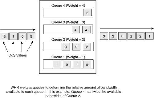 Throwing Packets out the WindowRecall from your early studies of networking technology how TCP windowing functions. A sender sends a single segment, and if the sender receives a successful acknowledgement from the receiver, the sender sends two segments (that is, a windows size of 2). If those two segments are successfully acknowledged, the sender sends four segments, and so on, increasing the window size exponentially. However, if a segment is dropped, the TCP flow goes into TCP slow start, where the window size is reduced to 1. The TCP flow then exponentially increases its window size until the window's size reaches half of the window size when congestion originally occurred. At that point the TCP flow's window size increases linearly. TCP slow start is relevant to QoS because when an interface's output queue is completely full, all newly arriving packets are discarded (that is, tail dropped), and all those TCP flows simultaneously go into TCP slow start. Note that the process of multiple TCP flows simultaneously entering TCP slow start is called global synchronization or TCP synchronization. When TCP synchronization occurs, a link's bandwidth is underutilized, resulting in wasted bandwidth. Random Early Detection (RED)To find a solution for global synchronization, we need look no further than my favorite Star Trek movie, Star Trek II: The Wrath of Khan. Remember the scene near the end of the movie where Spock is in the radiation chamber, and he's dying? He sacrificed his life to save the ship. Spock tells Kirk that this action was only logical, because the good of the many outweighs the good of the few, or the one. By the same logic, a QoS mechanism called random early detection (RED), sacrifices a few packets for the good of the many packets. To prevent a queue from completely filling to capacity, resulting in the tail drop of all packet flows, RED randomly discards a few packets. As a queue's depth (that is, the number of packets in the queue) increases, RED begins discarding packets more aggressively. Three parameters influence when RED discards a newly arriving packet:
The minimum threshold specifies the number of packets in a queue before the queue considers discarding packets. After the queue depth exceeds the minimum threshold, RED introduces the possibility that a packet will be discarded, and the probability of discard increases until the queue depth reaches the maximum threshold, as shown in Figure 6-15. After a queue depth exceeds the maximum threshold, all other packets attempting to enter the queue are discarded. Figure 6-15. Random Early Detection (RED) The probability of packet discard when the queue depth equals the maximum threshold is 1/(mark probability denominator). For example, if the mark probability denominator were set to 10, when the queue depth reached the maximum threshold, the probability of discard would be 1/10 (that is, a 10 percent chance of discard). The minimum threshold, maximum threshold, and mark probability denominator comprise a RED profile. As shown in Figure 6-16, there are three distinct ranges in a RED profile: 1) no drop, 2) random drop, and 3) full drop. The probability of discard at the maximum threshold equals 1/MPD. Therefore, in the figure, the probability of discard with the average queue depth of 45 packets equals 1/5 = .2 = 20 percent. Figure 6-16. RED Drop Ranges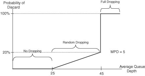 RED proves most useful on router interfaces where congestion is likely. For example, a WAN interface might be a good candidate for RED. Weighted RED (WRED)Cisco routers do not support RED, but fortunately Cisco routers support something better, WRED. Unlike RED, WRED creates a RED profile for each priority marking. For example, a packet marked with an IP Precedence value of 0 might have a minimum threshold of 20 packets, while a packet with an IP Precedence of 1 has a minimum threshold of 25 packets. In this example, packets with an IP Precedence of 0 would start to be discarded before packets with an IP Precedence of 1 as the queue begins to fill up. Explicit Congestion Notification (ECN)WRED discards packets, which is one way for the router to tell its neighbors that it's congested. However, Cisco routers can now indicate a congestion condition by signaling, using an approach called Explicit Congestion Notification (ECN). ECN uses the two last bits in an IP v4 header's ToS byte to indicate whether or not a device is ECN-capable and if so, whether or not congestion is being experienced, as shown in Figure 6-17. When ECN lets a router know that congestion is being experienced, the router can reduce its TCP transmission rate by transmitting fewer packets at a time before expecting an acknowledgement from the receiving device. Figure 6-17. Explicit Congestion Notification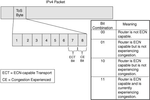 Cisco routers can use ECN as an extension to WRED and mark packets exceeding a specified queue threshold value. If the queue depth is at or below the WRED minimum threshold, the packets are sent normally, just as with WRED. Also, if the queue depth is above the WRED maximum threshold, all packets are dropped, just as with WRED. However, if the queue depth is currently somewhere in the range from just above the minimum threshold through the maximum threshold, one of three things might happen:
|
EAN: 2147483647
Pages: 138