Working with Ranges
The examples in this section demonstrate how to manipulate worksheet ranges with VBA.
Copying a range
Excel's macro recorder is useful not so much for generating usable code, but for discovering the names of relevant objects, methods , and properties. The code that's generated by the macro recorder isn't always the most efficient, but it can usually provide you with several clues.
For example, recording a simple copy-and-paste operation generates five lines of VBA code:
Sub Macro1() Range("A1").Select Selection.Copy Range("B1").Select ActiveSheet.Paste Application.CutCopyMode = False End Sub Notice that the generated code selects cell A1, copies it, and then selects cell B1 and performs the paste operation. But in VBA, it's not necessary to select an object to work with it. You would never learn this important point by mimicking the preceding recorded macro code, where two statements incorporate the Select method. This procedure can be replaced with the following much simpler routine, which doesn't select any cells . It also takes advantage of the fact that the Copy method can use an argument that represents the destination for the copied range:
Sub CopyRange() Range("A1").Copy Range("B1") End Sub Both of these macros assume that a worksheet is active and that the operation takes place on the active worksheet. To copy a range to a different worksheet or workbook, simply qualify the range reference for the destination. The following example copies a range from Sheet1 in File1.xlsx to Sheet2 in File2.xlsx . Because the references are fully qualified, this example works regardless of which workbook is active.
Sub CopyRange2() Workbooks("File1.xlsx").Sheets("Sheet1").Range("A1").Copy _ Workbooks("File2.xlsx").Sheets("Sheet2").Range("A1") End Sub Another way to approach this task is to use object variables to represent the ranges, as shown in the code that follows :
Sub CopyRange3() Dim Rng1 As Range, Rng2 As Range Set Rng1 = Workbooks("File1.xlsx").Sheets("Sheet1").Range("A1") Set Rng2 = Workbooks("File2.xlsx").Sheets("Sheet2").Range("A1") Rng1.Copy Rng2 End Sub As you might expect, copying is not limited to one single cell at a time. The following procedure, for example, copies a large range. Notice that the destination consists of only a single cell (which represents the upper-left cell for the destination).
Sub CopyRange4() Range("A1:C800").Copy Range("D1") End Sub Moving a range
The VBA instructions for moving a range are very similar to those for copying a range, as the following example demonstrates . The difference is that you use the Cut method instead of the Copy method. Note that you need to specify only the upper-left cell for the destination range.
The following example moves 18 cells (in A1:C6) to a new location, beginning at cell H1:
Sub MoveRange1() Range("A1:C6").Cut Range("H1") End Sub Copying a variably sized range
In many cases, you need to copy a range of cells, but you don't know the exact row and column dimensions of the range. For example, you might have a workbook that tracks weekly sales, and the number of rows changes weekly when you add new data.
Figure 11-1 shows a common type of worksheet. This range consists of several rows, and the number of rows changes each week. Because you don't know the exact range address at any given time, writing a macro to copy the range requires some additional coding.
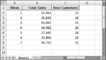
Figure 11-1: The number of rows in the data range changes every week.
The following macro demonstrates how to copy this range from Sheet1 to Sheet2 (beginning at cell A1). It uses the CurrentRegion property, which returns a Range object that corresponds to the block of cells around a particular cell (in this case, A1).
Sub CopyCurrentRegion2() Range("A1").CurrentRegion.Copy Sheets("Sheet2").Range("A1") End Sub | |
When you work with ranges, keep the following points in mind:
-
Your code doesn't need to select a range in order to work with it.
-
If your code does select a range, its worksheet must be active. You can use the Activate method of the Worksheets collection to activate a particular sheet.
-
The macro recorder doesn't always generate the most efficient code. Often, you can create your macro by using the recorder and then edit the code to make it more efficient.
-
It's a good idea to use named ranges in your VBA code. For example, referring to Range("Total") is better than Range("D45") . In the latter case, if you add a row above row 45, the cell address will change. You would then need to modify the macro so that it uses the correct range address (D46).
-
If you rely on the macro recorder when selecting ranges, make sure that you record the macro using relative references. Use the Developer
 Code
Code  Use Relative References control.
 -
When running a macro that works on each cell in the current range selection, the user might select entire columns or rows. In most cases, you don't want to loop through every cell in the selection. Your macro should create a subset of the selection consisting of only the nonblank cells. See "Looping through a selected range efficiently ," later in this chapter.
-
Excel allows multiple selections. For example, you can select a range, press Ctrl, and select another range. You can test for this in your macro and take appropriate action. See "Determining the type of selected range," later in this chapter.
| |
| Note | Using the CurrentRegion property is equivalent to choosing the Home |
Selecting or otherwise identifying various types of ranges
Much of the work that you will do in VBA will involve working with ranges - either selecting a range or identifying a range so that you can do something with the cells.
In addition to the CurrentRegion property (which I discussed earlier), you should also be aware of the End method of the Range object. The End method takes one argument, which determines the direction in which the selection is extended. The following statement selects a range from the active cell to the last non-empty cell:
Range(ActiveCell, ActiveCell.End(xlDown)).Select
As you might expect, three other constants simulate key combinations in the other directions: xlUp , xlToLeft , and xlToRight .
| Caution | Be careful when using the End method. If the active cell is at the perimeter of a range or if the range contains one or more empty cells, the End method may not produce the desired results. |
| CD-ROM | The companion CD-ROM includes a workbook that demonstrates several common types of range selections. When you open this workbook, named |
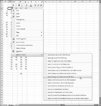
Figure 11-2: This workbook uses a custom shortcut menu to demonstrate how to select variably sized ranges by using VBA.
The following macro is in the example workbook. The SelectCurrentRegion macro simulates pressing Ctrl+Shift+*.
Sub SelectCurrentRegion() ActiveCell.CurrentRegion.Select End Sub
Often, you won't want to actually select the cells. Rather, you'll want to work with them in some way (for example, format them). The cell-selecting procedures can easily be adapted. The following procedure was adapted from SelectCurrentRegion . This procedure doesn't select cells; it applies formatting to the range that's defined as the current region around the active cell. The other procedures in the example workbook can also be adapted in this manner.
Sub FormatCurrentRegion() ActiveCell.CurrentRegion.Font.Bold = True End Sub
Prompting for a cell value
The following procedure demonstrates how to ask the user for a value and then insert it into cell A1 of the active worksheet:
Sub GetValue1() Range("A1").Value = InputBox("Enter the value") End Sub Figure 11-3 shows how the input box looks.
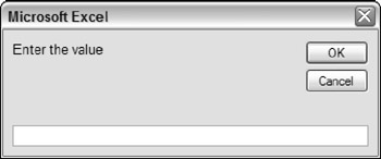
Figure 11-3: The InputBox function gets a value from the user to be inserted into a cell.
This procedure has a problem, however. If the user clicks the Cancel button in the input box, the procedure deletes any data already in the cell. The following modification takes no action if the Cancel button is clicked:
Sub GetValue2() Dim UserEntry As Variant UserEntry = InputBox("Enter the value") If UserEntry <> "" Then Range("A1").Value = UserEntry End Sub In many cases, you'll need to validate the user's entry in the input box. For example, you may require a number between 1 and 12. The following example demonstrates one way to validate the user's entry. In this example, an invalid entry is ignored, and the input box is displayed again. This cycle keeps repeating until the user enters a valid number or clicks Cancel.
Sub GetValue3() Dim UserEntry As Variant Dim Msg As String Const MinVal As Integer = 1 Const MaxVal As Integer = 12 Msg = "Enter a value between " & MinVal & " and " & MaxVal Do UserEntry = InputBox(Msg) If UserEntry = "" Then Exit Sub If IsNumeric(UserEntry) Then If UserEntry >= MinVal And UserEntry <= MaxVal Then Exit Do End If Msg = "Your previous entry was INVALID." Msg = Msg & vbNewLine Msg = Msg & "Enter a value between " & MinVal & " and " & MaxVal Loop ActiveSheet.Range("A1").Value = UserEntry End Sub As you can see in Figure 11-4, the code also changes the message displayed if the user makes an invalid entry.
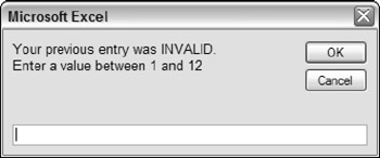
Figure 11-4: Validate a user's entry with the VBA InputBox function.
| CD-ROM | The three GetValue procedures are available on the companion CD-ROM. The filename is |
Entering a value in the next empty cell
A common requirement is to enter a value into the next empty cell in a column or row. The following example prompts the user for a name and a value and then enters the data into the next empty row (see Figure 11-5).
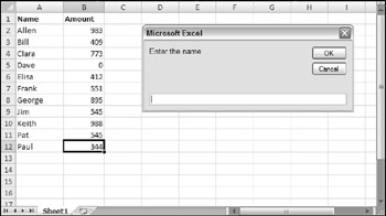
Figure 11-5: A macro for inserting data into the next empty row in a worksheet.
Sub GetData() Dim NextRow As Long Dim Entry1 As String, Entry2 As String Do 'Determine next empty row NextRow = Cells(Rows.Count, 1).End(xlUp).Row + 1 ' Prompt for the data Entry1 = InputBox("Enter the name") If Entry1 = "" Then Exit Sub Entry2 = InputBox("Enter the amount") If Entry2 = "" Then Exit Sub ' Write the data Cells(NextRow, 1) = Entry1 Cells(NextRow, 2) = Entry2 Loop End Sub To keep things simple, this procedure doesn't perform any validation. Notice that the loop continues indefinitely. I use Exit Sub statements to get out of the loop when the user clicks Cancel in the input box.
| CD-ROM | The GetData procedure is available on the companion CD-ROM. The filename is next empty cell.xlsm . |
Notice the statement that determines the value of the NextRow variable. If you don't understand how this works, try the manual equivalent: Activate the last cell in column A, press End, and then press the up-arrow key. At this point, the last nonblank cell in column A will be selected. The Row property returns this row number, and it is incremented by 1 in order to get the row of the cell below it (the next empty row). Rather than hard-code the last cell in column A, I used Rows.Count so this procedure will work with previous versions of Excel (which have fewer rows).
Note that this technique of selecting the next empty cell has a slight glitch. If the column is completely empty, it will calculate row 2 as the next empty row. It would be fairly easy to write additional code to account for this possibility.
Pausing a macro to get a user-selected range
In some situations, you may need an interactive macro. For example, you can create a macro that pauses while the user specifies a range of cells. The procedure in this section describes how to do this with Excel's InputBox method.
| Note | Do not confuse Excel's InputBox method with VBA's InputBox function. Although these two items have the same name, they are not the same. |
The Sub procedure that follows demonstrates how to pause a macro and let the user select a range. The code then inserts a formula into each cell of the specified range.
Sub GetUserRange() Dim UserRange As Range Prompt = "Select a range for the random numbers." Title = "Select a range" ' Display the Input Box On Error Resume Next Set UserRange = Application.InputBox(_ Prompt:=Prompt, _ Title:=Title, _ Default:=ActiveCell.Address, _ Type:=8) 'Range selection On Error GoTo 0 ' Was the Input Box canceled? If UserRange Is Nothing Then MsgBox "Canceled." Else UserRange.Formula = "=RAND()" End If End Sub
The input box is shown in Figure 11-6.
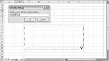
Figure 11-6: Use an input box to pause a macro.
| CD-ROM | This example, named |
Specifying a Type argument of 8 for the InputBox method is the key to this procedure. Also, note the use of On Error Resume Next . This statement ignores the error that occurs if the user clicks the Cancel button. If so, the UserRange object variable is not defined. This example displays a message box with the text Canceled . If the user clicks OK, the macro continues. Using On Error GoTo 0 resumes normal error handling.
By the way, it's not necessary to check for a valid range selection. Excel takes care of this for you.
| Caution | Make sure that screen updating is not turned off when you use the InputBox method to select a range. Otherwise, you won't be able to make a worksheet selection. Use the ScreenUpdating property of the Application object to control screen updating while a macro is running. |
Counting selected cells
You can create a macro that works with the selected range of cells. Use the Count property of the Range object to determine how many cells are contained in a range selection (or any range, for that matter). For example, the following statement displays a message box that contains the number of cells in the current selection:
MsgBox Selection.Count
| Caution | With the larger worksheet size in Excel 2007, the Count property can generate an error. The Count property uses the Long data type, so the largest value that it can store is 2,147,483,647. For example, if the user selects 2,048 complete columns (2,147,483,648 cells), the Count property generates an error. Fortunately, Microsoft added a new property: CountLarge . CountLarge uses the Double data type, which can handle values up to 1.79+E ˆ˜ 308. Bottom line? In the vast majority of situations, the Count property will work fine. If there's a chance that you may need to count more cells (such as all cells in a worksheet), use CountLarge instead of Count . |
If the active sheet contains a range named data , the following statement assigns the number of cells in the data range to a variable named CellCount :
CellCount = Range("data").Count You can also determine how many rows or columns are contained in a range. The following expression calculates the number of columns in the currently selected range:
Selection.Columns.Count
And, of course, you can also use the Rows property to determine the number of rows in a range. The following statement counts the number of rows in a range named data and assigns the number to a variable named RowCount :
RowCount = Range("data").Rows.Count Determining the type of selected range
Excel supports several types of range selections:
-
A single cell
-
A contiguous range of cells
-
One or more entire columns
-
One or more entire rows
-
The entire worksheet
-
Any combination of the above (that is, a multiple selection)
As a result, when your VBA procedure processes a user-selected range, you can't make any presumptions about what that range might be.
In the case of a multiple range selection, the Range object comprises separate areas. To determine whether a selection is a multiple selection, use the Areas method, which returns an Areas collection. This collection represents all the ranges within a multiple range selection.
You can use an expression like the following to determine whether a selected range has multiple areas:
NumAreas = Selection.Areas.Count
If the NumAreas variable contains a value greater than 1, the selection is a multiple selection.
Following is a function named AreaType , which returns a text string that describes the type of range selection.
Function AreaType(RangeArea As Range) As String ' Returns the type of a range in an area Select Case True Case RangeArea.Cells.CountLarge = 1 AreaType = "Cell" Case RangeArea.CountLarge = Cells.CountLarge AreaType = "Worksheet" Case RangeArea.Rows.Count = Cells.Rows.Count AreaType = "Column" Case RangeArea.Columns.Count = Cells.Columns.Count AreaType = "Row" Case Else AreaType = "Block" End Select End Function
This function accepts a Range object as its argument and returns one of five strings that describe the area: Cell , Worksheet , Column , Row , or Block . The function uses a Select Case construct to determine which of five comparison expressions is True . For example, if the range consists of a single cell, the function returns Cell . If the number of cells in the range is equal to the number of cells in the worksheet, it returns Worksheet . If the number of rows in the range equals the number of rows in the worksheet, it returns Column . If the number of columns in the range equals the number of columns in the worksheet, the function returns Row . If none of the Case expressions is True , the function returns Block .
Notice that I used the CountLarge property when counting cells. As I noted previously in this chapter, the number of selected cells in Excel 2007 could potentially exceed the limit of the Count property.
| CD-ROM | This example is available on the companion CD-ROM in a file named |
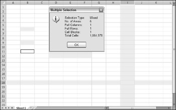
Figure 11-7: A VBA procedure analyzes the currently selected range.
| Note | You might be surprised to discover that Excel allows multiple selections to be identical. For example, if you hold down Ctrl and click five times in cell A1, the selection will have five identical areas. The RangeDescription procedure takes this into account and does not count the same cell multiple times. |
Looping through a selected range efficiently
A common task is to create a macro that evaluates each cell in a range and performs an operation if the cell meets a certain criterion. The procedure that follows is an example of such a macro. The ColorNegative procedure sets the cell's background color to red for cells that contain a negative value. For non-negative value cells, it sets the background color to none.
| Note | This example is for educational purposes only. Using Excel's conditional formatting is a much better approach. |
Sub ColorNegative() ' Makes negative cells red Dim cell As Range If TypeName(Selection) <> "Range" Then Exit Sub Application.ScreenUpdating = False For Each cell In Selection If cell.Value < 0 Then cell.Interior.Color = RGB(255, 0, 0) Else cell.Interior.Color = xlNone End If Next cell End Sub
The ColorNegative procedure certainly works, but it has a serious flaw. For example, what if the used area on the worksheet were small, but the user selects an entire column? Or ten columns? Or the entire worksheet? There's no need to process all of those empty cells, and the user would probably give up before all the cells were evaluated.
A better solution ( ColorNegative2 ) follows. In this revised procedure, I create a Range object variable, WorkRange , which consists of the intersection of the selected range and the worksheet's used range. Figure 11-8 shows an example; the entire column D is selected (1,048,576 cells). The worksheet's used range, however, consists of the range B2:I18. Therefore, the intersection of these ranges is D2:D18, which is a much smaller range than the original selection. The time difference between processing 16 cells versus processing 1,048,576 cells is significant.
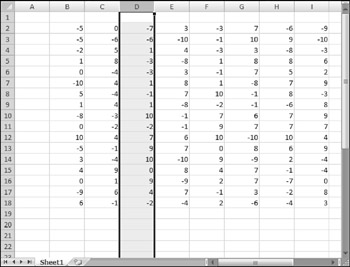
Figure 11-8: Using the intersection of the used range and the selected ranged results in fewer cells to process.
Sub ColorNegative2() ' Makes negative cells red Dim WorkRange As Range Dim cell As Range If TypeName(Selection) <> "Range" Then Exit Sub Application.ScreenUpdating = False Set WorkRange = Application.Intersect(Selection, _ ActiveSheet.UsedRange) For Each cell In WorkRange If cell.Value < 0 Then cell.Interior.Color = RGB(255, 0, 0) Else cell.Interior.Color = xlNone End If Next cell End Sub
The ColorNegative2 procedure is an improvement, but it's still not as efficient as it could be because it processes empty cells. A third revision, ColorNegative3 , is quite a bit longer, but it's much more efficient. I use the SpecialCells method to generate two subsets of the selection: One subset ( ConstantCells ) includes only the cells with numeric constants; the other subset ( FormulaCells ) includes only the cells with numeric formulas. The code processes the cells in these subsets by using two For Each-Next constructs. The net effect: Only non-blank, non-text cells are evaluated, thus speeding up the macro considerably.
Sub ColorNegative3() ' Makes negative cells red Dim FormulaCells As Range, ConstantCells As Range Dim cell As Range If TypeName(Selection) <> "Range" Then Exit Sub Application.ScreenUpdating = False ' Create subsets of original selection On Error Resume Next Set FormulaCells = Selection.SpecialCells(xlFormulas, xlNumbers) Set ConstantCells = Selection.SpecialCells(xlConstants, xlNumbers) On Error GoTo 0 ' Process the formula cells If Not FormulaCells Is Nothing Then For Each cell In FormulaCells If cell.Value < 0 Then cell.Interior.Color = RGB(255, 0, 0) Else cell.Interior.Color = xlNone End If Next cell End If ' Process the constant cells If Not ConstantCells Is Nothing Then For Each cell In ConstantCells If cell.Value < 0 Then cell.Interior.Color = RGB(255, 0, 0) Else cell.Interior.Color = xlNone End If Next cell End If End Sub
| Note | The On Error statement is necessary because the SpecialCells method generates an error if no cells qualify. |
| CD-ROM | A workbook that contains the three ColorNegative procedures is available on the companion CD-ROM. The file is named |
Deleting all empty rows
The following procedure deletes all empty rows in the active worksheet. This routine is fast and efficient because it doesn't check all rows. It checks only the rows in the used range, which is determined by using the UsedRange property of the Worksheet object.
Sub DeleteEmptyRows() Dim LastRow As Long Dim r As Long Dim Counter As Long Application.ScreenUpdating = False LastRow = ActiveSheet.UsedRange.Rows.Count + _ ActiveSheet.UsedRange.Rows(1).Row - 1 For r = LastRow To 1 Step -1 If Application.WorksheetFunction.CountA(Rows(r)) = 0 Then Rows(r).Delete Counter = Counter + 1 End If Next r Application.ScreenUpdating = True MsgBox Counter & " empty rows were deleted." End Sub
The first step is to determine the last used row and then assign this row number to the LastRow variable. This is not as simple as you might think because the used range may or may not begin in row 1. Therefore, LastRow is calculated by determining the number of rows in the used range, adding the first row number in the used range, and subtracting 1.
The procedure uses Excel's COUNTA worksheet function to determine whether a row is empty. If this function returns for a particular row, the row is empty. Notice that the procedure works on the rows from bottom to top and also uses a negative step value in the For-Next loop. This is necessary because deleting rows causes all subsequent rows to move up in the worksheet. If the looping occurred from top to bottom, the counter within the loop would not be accurate after a row is deleted.
The macro uses another variable, Counter , to keep track of how many rows were deleted. This number is displayed in a message box when the procedure ends.
| CD-ROM | A workbook that contains this example is available on the companion CD-ROM in a file named |
Duplicating rows a variable number of times
The example in this section demonstrates how to use VBA to create duplicates of a row. Figure 11-9 shows a worksheet for an office raffle. Column A contains the name, and column B contains the number of tickets purchased by each person. Column C contains a random number (generated by the RAND function). The winner will be determined by sorting the data based on column 3 (the highest random number wins).
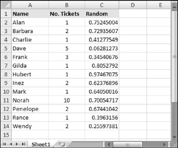
Figure 11-9: The goal is to duplicate rows based on the value in column B.
The goal is to duplicate the rows so each person will have a row for each ticket purchased. For example, Barbara purchased two tickets, so she should have two rows. The procedure to insert the new rows is shown here:
Sub DupeRows() Dim cell As Range ' 1st cell with number of tickets Set cell = Range("B2") Do While Not IsEmpty(cell) If cell > 1 Then Range(cell.Offset(1, 0), cell.Offset(cell.Value - 1, _ 0)).EntireRow.Insert Range(cell, cell.Offset(cell.Value - 1, 1)).EntireRow.FillDown End If Set cell = cell.Offset(cell.Value, 0) Loop End Sub The cell object variable is initialized to cell B2, the first cell that has a number. The loop inserts new rows and then copies the row using the FillDown method. The cell variable is incremented to the next person, and the loop continues until an empty cell is encountered . Figure 11-10 shows the worksheet after running this procedure.
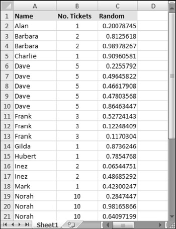
Figure 11-10: New rows were added, according to the value in column B.
| CD-ROM | A workbook that contains this example is available on the companion CD-ROM. The file is named |
Determining whether a range is contained in another range
The following InRange function accepts two arguments, both Range objects. The function returns True if the first range is contained in the second range.
Function InRange(rng1, rng2) As Boolean ' Returns True if rng1 is a subset of rng2 InRange = False If rng1.Parent.Parent.Name = rng2.Parent.Parent.Name Then If rng1.Parent.Name = rng2.Parent.Name Then If Union(rng1, rng2).Address = rng2.Address Then InRange = True End If End If End If End Function
The InRange function may appear a bit more complex than it needs to be because the code needs to ensure that the two ranges are in the same worksheet and workbook. Notice that the procedure uses the Parent property, which returns an object's container object. For example, the following expression returns the name of the worksheet for the rng1 object reference:
rng1.Parent.Name
The following expression returns the name of the workbook for rng1 :
rng1.Parent.Parent.Name
VBA's Union function returns a Range object that represents the union of two Range objects. The union consists of all the cells from both ranges. If the address of the union of the two ranges is the same as the address of the second range, the first range is contained within the second range.
| CD-ROM | A workbook that contains this function is available on the companion CD-ROM in a file named |
Determining a cell's data type
Excel provides a number of built-in functions that can help determine the type of data contained in a cell. These include ISTEXT, ISLOGICAL, and ISERROR. In addition, VBA includes functions such as IsEmpty , IsDate , and IsNumeric .
The following function, named CellType , accepts a range argument and returns a string ( Blank , Text , Logical , Error , Date , Time , or Number ) that describes the data type of the upper-left cell in the range. You can use this function in a worksheet formula or from another VBA procedure.
Function CellType(Rng) ' Returns the cell type of the upper left ' cell in a range Dim TheCell As Range Set TheCell = Rng.Range("A1") Select Case True Case IsEmpty(TheCell) CellType = "Blank" Case Application.IsText(TheCell) CellType = "Text" Case Application.IsLogical(TheCell) CellType = "Logical" Case Application.IsErr(TheCell) CellType = "Error" Case IsDate(TheCell) CellType = "Date" Case InStr(1, TheCell.Text, ":") <> 0 CellType = "Time" Case IsNumeric(TheCell) CellType = "Number" End Select End Function Notice the use of the Set TheCell statement.. The CellType function accepts a range argument of any size, but this statement causes it to operate on only the upper-left cell in the range (which is represented by the TheCell variable).
| CD-ROM | A workbook that contains this function is available on the companion CD-ROM. The file is named |
Reading and writing ranges
Many VBA tasks involve transferring values either from an array to a range or from a range to an array. For some reason, Excel reads from ranges much faster than it writes to ranges. The WriteReadRange procedure that follows demonstrates the relative speeds of writing and reading a range.
This procedure creates an array and then uses For-Next loops to write the array to a range and then read the range back into the array. It calculates the time required for each operation by using the Excel Timer function.
Sub WriteReadRange() Dim MyArray() Dim Time1 As Double Dim NumElements As Long, i As Long Dim WriteTime As String, ReadTime As String Dim Msg As String NumElements = 60000 ReDim MyArray(1 To NumElements) ' Fill the array For i = 1 To NumElements MyArray(i) = i Next i ' Write the array to a range Time1 = Timer For i = 1 To NumElements Cells(i, 1) = MyArray(i) Next i WriteTime = Format(Timer - Time1, "00:00") ' Read the range into the array Time1 = Timer For i = 1 To NumElements MyArray(i) = Cells(i, 1) Next i ReadTime = Format(Timer - Time1, "00:00") ' Show results Msg = "Write: " & WriteTime Msg = Msg & vbCrLf Msg = Msg & "Read: " & ReadTime MsgBox Msg, vbOKOnly, NumElements & " Elements" End Sub
On my system, it took 12 seconds to write a 60,000-element array to a range but only 1 second to read the range into an array.
A better way to write to a range
The example in the preceding section uses a For-Next loop to transfer the contents of an array to a worksheet range. In this section, I demonstrate a more efficient way to accomplish this.
Start with the example that follows, which illustrates the most obvious (but not the most efficient) way to fill a range. This example uses a For-Next loop to insert its values in a range.
Sub LoopFillRange() ' Fill a range by looping through cells Dim CellsDown As Long, CellsAcross As Integer Dim CurrRow As Long, CurrCol As Integer Dim StartTime As Double Dim CurrVal As Long ' Get the dimensions CellsDown = InputBox("How many cells down?") If CellsDown = 0 Then Exit Sub CellsAcross = InputBox("How many cells across?") If CellsAcross = 0 Then Exit Sub ' Record starting time StartTime = Timer ' Loop through cells and insert values CurrVal = 1 Application.ScreenUpdating = False For CurrRow = 1 To CellsDown For CurrCol = 1 To CellsAcross ActiveCell.Offset(CurrRow - 1, _ CurrCol - 1).Value = CurrVal CurrVal = CurrVal + 1 Next CurrCol Next CurrRow ' Display elapsed time Application.ScreenUpdating = True MsgBox Format(Timer - StartTime, "00.00") & " seconds" End Sub The example that follows demonstrates a much faster way to produce the same result. This code inserts the values into an array and then uses a single statement to transfer the contents of an array to the range.
Sub ArrayFillRange() ' Fill a range by transferring an array Dim CellsDown As Long, CellsAcross As Integer Dim i As Long, j As Integer Dim StartTime As Double Dim TempArray() As Long Dim TheRange As Range Dim CurrVal As Long ' Get the dimensions CellsDown = InputBox("How many cells down?") If CellsDown = 0 Then Exit Sub CellsAcross = InputBox("How many cells across?") If CellsAcross = 0 Then Exit Sub ' Record starting time StartTime = Timer ' Redimension temporary array ReDim TempArray(1 To CellsDown, 1 To CellsAcross) ' Set worksheet range Set TheRange = ActiveCell.Range(Cells(1, 1), _ Cells(CellsDown, CellsAcross)) ' Fill the temporary array CurrVal = 0 Application.ScreenUpdating = False For i = 1 To CellsDown For j = 1 To CellsAcross TempArray(i, j) = CurrVal + 1 CurrVal = CurrVal + 1 Next j Next i ' Transfer temporary array to worksheet TheRange.Value = TempArray ' Display elapsed time Application.ScreenUpdating = True MsgBox Format(Timer - StartTime, "00.00") & " seconds" End Sub On my system, using the loop method to fill a 500 — 256 “cell range (128,000 cells) took 12.81 seconds. The array transfer method took only 0.20 seconds to generate the same results - more than 60 times faster! The moral of this story? If you need to transfer large amounts of data to a worksheet, avoid looping whenever possible.
| CD-ROM | A workbook that contains the WriteReadRange , LoopFillRange , and ArrayFillRange procedures is available on the companion CD-ROM. The file is named |
Transferring one-dimensional arrays
The example in the preceding section involves a two-dimensional array, which works out nicely for row-and-column-based worksheets.
When transferring a one-dimensional array to a range, the range must be horizontal - that is, one row with multiple columns. If you need the data in a vertical range instead, you must first transpose the array to make it vertical. You can use Excel's TRANSPOSE function to do this. The following example transfers a 100-element array to a vertical worksheet range (A1:A100):
Range("A1:A100").Value = Application.WorksheetFunction.Transpose(MyArray) Transferring a range to a variant array
This section discusses yet another way to work with worksheet data in VBA. The following example transfers a range of cells to a two-dimensional variant array. Then message boxes display the upper bounds for each dimension of the variant array.
Sub RangeToVariant() Dim x As Variant x = Range("A1:L600").Value MsgBox UBound(x, 1) MsgBox UBound(x, 2) End Sub In this example, the first message box displays 600 (the number of rows in the original range), and the second message box displays 12 (the number of columns). You'll find that transferring the range data to a variant array is virtually instantaneous.
The following example reads a range (named data ) into a variant array, performs a simple multiplication operation on each element in the array, and then transfers the variant array back to the range.
Sub RangeToVariant2() Dim As Variant Dim r As Long, c As Integer ' Read the data into the variant x = Range("data").Value ' Loop through the variant array For r = 1 To UBound(x, 1) For c = 1 To UBound(x, 2) ' Multiply by 2 x(r, c) = x(r, c) * 2 Next c Next r ' Transfer the variant back to the sheet Range("data") = End Sub You'll find that this procedure runs amazingly fast.
| CD-ROM | A workbook that contains this example is available on the companion CD-ROM. The file is named |
Selecting cells by value
The example in this section demonstrates how to select cells based on their value. Oddly enough, Excel does not provide a direct way to perform this operation. My SelectByValue procedure follows. In this example, the code selects cells that contain a negative value, but this can be changed easily.
Sub SelectByValue() Dim Cell As Object Dim FoundCells As Range Dim WorkRange As Range If TypeName(Selection) <> "Range" Then Exit Sub ' Check all or selection? If Selection.CountLarge = 1 Then Set WorkRange = ActiveSheet.UsedRange Else Set WorkRange = Application.Intersect(Selection, ActiveSheet.UsedRange) End If ' Reduce the search to numeric cells only On Error Resume Next Set WorkRange = WorkRange.SpecialCells(xlConstants, xlNumbers) If WorkRange Is Nothing Then Exit Sub On Error GoTo 0 ' Loop through each cell, add to the FoundCells range if it qualifies For Each Cell In WorkRange If Cell.Value < 0 Then If FoundCells Is Nothing Then Set FoundCells = Cell Else Set FoundCells = Union(FoundCells, Cell) End If End If Next Cell ' Show message, or select the cells If FoundCells Is Nothing Then MsgBox "No cells qualify." Else FoundCells.Select End If End Sub
The procedure starts by checking the selection. If it's a single cell, then the entire worksheet is searched. If the selection is at least two cells, then only the selected range is searched. The range to be searched is further refined by using the SpecialCells method to create a Range object that consists only of the numeric constants.
The code within the For-Next loop examines the cell's value. If it meets the criterion (less than 0), then the cell is added to the FoundCells Range object by using the Union method. Note that you can't use the Union method for the first cell. If the FoundCells range contains no cells, attempting to use the Union method will generate an error. Therefore, the code checks whether FoundCells is Nothing .
When the loop ends, the FoundCells object will consist of the cells that meet the criterion (or will be Nothing if no cells were found). If no cells are found, a message box appears. Otherwise, the cells are selected.
| CD-ROM | This example is available on the companion CD-ROM. The file is named select by value.xlsm . |
Copying a noncontiguous range
If you've ever attempted to copy a noncontiguous range selection, you discovered that Excel doesn't support such an operation. Attempting to do so brings up an error message: That command cannot be used on multiple selections .
When you encounter a limitation in Excel, you can often circumvent it by creating a macro. The example is this section is a VBA procedure that allows you to copy a multiple selection to another location.
Sub CopyMultipleSelection() Dim SelAreas() As Range Dim PasteRange As Range Dim UpperLeft As Range Dim NumAreas As Long, i As Long Dim TopRow As Long, LeftCol As Long Dim RowOffset As Long, ColOffset As Long If TypeName(Selection) <> "Range" Then Exit Sub ' Store the areas as separate Range objects NumAreas = Selection.Areas.Count ReDim SelAreas(1 To NumAreas) For i = 1 To NumAreas Set SelAreas(i) = Selection.Areas(i) Next ' Determine the upper-left cell in the multiple selection TopRow = ActiveSheet.Rows.Count LeftCol = ActiveSheet.Columns.Count For i = 1 To NumAreas If SelAreas(i).Row < TopRow Then TopRow = SelAreas(i).Row If SelAreas(i).Column < LeftCol Then LeftCol = SelAreas(i).Column Next Set UpperLeft = Cells(TopRow, LeftCol) ' Get the paste address On Error Resume Next Set PasteRange = Application.InputBox _ (Prompt:="Specify the upper-left cell for the paste range:", _ Title:="Copy Multiple Selection", _ Type:=8) On Error GoTo 0 ' Exit if canceled If TypeName(PasteRange) <> "Range" Then Exit Sub ' Make sure only the upper-left cell is used Set PasteRange = PasteRange.Range("A1") ' Copy and paste each area For i = 1 To NumAreas RowOffset = SelAreas(i).Row - TopRow ColOffset = SelAreas(i).Column - LeftCol SelAreas(i).Copy PasteRange.Offset(RowOffset, ColOffset) Next i End Sub Figure 11-11 shows the prompt to select the destination location.
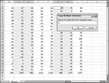
Figure 11-11: Using Excel's InputBox method to prompt for a cell location.
| CD-ROM | The companion CD-ROM contains a workbook with this example, plus another version that warns the user if data will be overwritten. The file is named |
EAN: 2147483647
Pages: 319