Using Single-Cell Array Formulas

The examples in the previous section all used a multicell array formula-a single array formula entered into a range of cells. The real power of using arrays becomes apparent when you use single-cell array formulas. This section contains examples of array formulas that occupy a single cell.

Counting Characters in a Range

Suppose you have a range of cells that contains text entries (see Figure 14-13). If you need to get a count of the total number of characters in that range, the "traditional" method involves creating a formula like the one that follows and copying it down the column:

 =LEN(A1) 

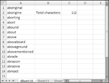
Figure 14-13: The goal is to count the number of characters in a range of text.

Then, you use a SUM formula to calculate the sum of the values returned by the intermediate formulas.

The following array formula does the job without using any intermediate formulas:

 {=SUM(LEN(A1:A14))} 

The array formula uses the LEN function to create a new array (in memory) that consists of the number of characters in each cell of the range. In this case, the new array is

 {10,9,8,5,6,5,5,10,11,14,6,8,8,7} 

The array formula is then reduced to the following:

 =SUM({10,9,8,5,6,5,5,10,11,14,6,8,8,7}) 

Summing the Three Smallest Values in a Range

The following formula returns the sum of the three smallest values in a range named Data:

 {=SUM(SMALL(Data,{1,2,3}))} 

The function uses an array constant as the second argument for the SMALL function. This generates a new array, which consists of the three smallest values in the range. This array is then passed to the SUM function, which returns the sum of the values in the new array.

Figure 14-14 shows an example in which the range A1:A10 is named Data. The SMALL function is evaluated three times, each time with a different second argument. The first time, the SMALL function has a second argument of 1, and it returns –5. The second time, the second argument for the SMALL function is 2, and it returns 0 (the second-smallest value in the range). The third time, the SMALL function has a second argument of 3, and returns the third-smallest value of 2.

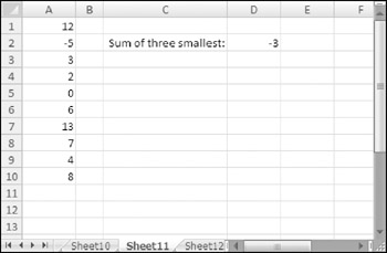
Figure 14-14: An array formula returns the sum of the three smallest values in A1:A10.

Therefore, the array that's passed to the SUM function is

 {-5,0,2) 

The formula returns the sum of the array (–3).

Counting Text Cells in a Range

The following array formula uses the IF function to examine each cell in a range. It then creates a new array (of the same size and dimensions as the original range) that consists of 1s and 0s, depending on whether the cell contains text. This new array is then passed to the SUM function, which returns the sum of the items in the array. The result is a count of the number of text cells in the range.

 {=SUM(IF(ISTEXT(A1:D5),1,0))} 

Cross Ref 

This general array formula type (that is, an IF function nested in a SUM function) is very useful for counting. Refer to Chapter 7 for additional examples.

Figure 14-15 shows an example of the preceding formula in cell C8. The array created by the IF function is as follows:

 {0,1,1,1;1,0,0,0;1,0,0,0;1,0,0,0;1,0,0,0}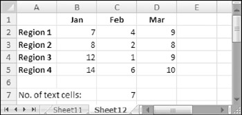 

Figure 14-15: An array formula returns the number of text cells in the range.

TRUE and FALSE in Array Formulas

When your arrays return Boolean values (True or False), you must coerce these Boolean values into numbers. Excel's SUM function ignores Booleans, but you can still perform mathematical operation on them. In Excel, True is equivalent to a value of 1 and False to a value of 0. Converting True and False to these values ensures the SUM function treats them appropriately.

You can use three mathematical operations to convert True and False to numbers without changing their values, called identity operations.

• Multiply by 1: (x * 1 = x)

• Add zero: (x + 0 = x)

• Double negative: (–– x = x)

Applying any of these operations to a Boolean value will cause Excel to convert it to a number. The following formulas all return the same answer:

 {=SUM(ISTEXT(A1:D5)*1)} {=SUM(ISTEXT(A1:D5)+0)} {=SUM(--ISTEXT(A1:D5))} 

There is no "best" way to convert Boolean values to numbers. Pick a method that you like and use that. However, be aware of all three methods so that you can identify them in other people's spreadsheets.

Notice that this array contains four rows of three elements (the same dimensions as the range).

A variation on this formula follows:

 {=SUM(ISTEXT(A1:D5)*1)} 

This formula eliminates the need for the IF function and takes advantage of the fact that

 TRUE * 1 = 1 

and

 FALSE * 1 = 0 

Eliminating Intermediate Formulas

One of the main benefits of using an array formula is that you can eliminate intermediate formulas in your worksheet. This makes your worksheet more compact and eliminates the need to display irrelevant calculations. Figure 14-16 shows a worksheet that contains pre-test and post-test scores for students. Column D contains formulas that calculate the changes between the pre-test and the post-test scores. Cell D17 contains the following formula, which calculates the average of the values in column D:

 =AVERAGE(D2:D15) 

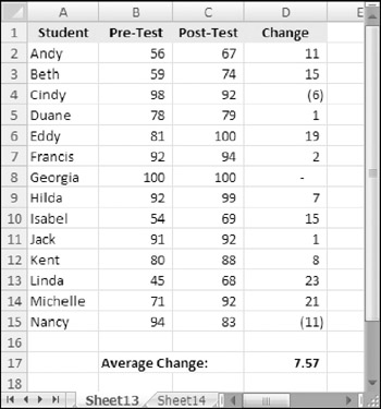
Figure 14-16: Without an array formula, calculating the average change requires intermediate formulas in column D.

With an array formula, you can eliminate column D. The following array formula calculates the average of the changes but does not require the formulas in column D:

 {=AVERAGE(C2:C15-B2:B15)} 

How does it work? The formula uses two arrays, the values of which are stored in two ranges (B2:B15 and C2:C15). The formula creates a new array that consists of the differences between each corresponding element in the other arrays. This new array is stored in Excel's memory, not in a range. The AVERAGE function then uses this new array as its argument and returns the result.

The new array consists of the following elements:

 {11,15,-6,1,19,2,0,7,15,1,8,23,21,-11} 

The formula, therefore, is reduced to the following:

 =AVERAGE({11,15,-6,1,19,2,0,7,15,1,8,23,21,-11}) 

You can use additional array formulas to calculate other measures for the data in this example. For instance, the following array formula returns the largest change (that is, the greatest improvement). This formula returns 23, which represents Linda's test scores:

 {=MAX(C2:C15-B2:B15)} 

The following array formula returns the smallest change (that is, the least improvement). This formula returns –11, which represents Nancy's test scores.

 {=MIN(C2:C15-B2:B15)} 

Using an Array in Lieu of a Range Reference

If your formula uses a function that requires a range reference, you may be able to replace that range reference with an array constant. This is useful in situations in which the values in the referenced range do not change.

Note 

A notable exception to using an array constant in place of a range reference in a function is with the database functions that use a reference to a criteria range (for example, DSUM). Unfortunately, using an array constant instead of a reference to a criteria range does not work.

Figure 14-17 shows a worksheet that uses a lookup table to display a word that corresponds to an integer. For example, looking up a value of 9 returns Nine from the lookup table in D1:E10. The formula in cell C1 is

 =VLOOKUP(B1,D1:E10,2,FALSE) 

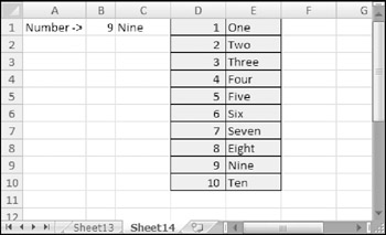
Figure 14-17: You can replace the lookup table in D1:E10 with an array constant.

You can use a two-dimensional array in place of the lookup range. The following formula returns the same result as the previous formula, but it does not require the lookup range in D1:E1:

 =VLOOKUP(B1,{1,"One";2,"Two";3,"Three";4,"Four";5,"Five"; 6,"Six";7,"Seven";8,"Eight";9,"Nine";10,"Ten"},2,FALSE)