Using Multicell Array Formulas

This section contains examples that demonstrate additional features of multicell array formulas (array formulas that are entered into a range of cells). These features include creating arrays from values, performing operations, using functions, transposing arrays, and generating consecutive integers.

Creating an Array from Values in a Range

The following array formula creates an array from a range of cells. Figure 14-7 shows a workbook with some data entered into A1:C4. The range D8:F11 contains a single array formula:

 {=A1:C4}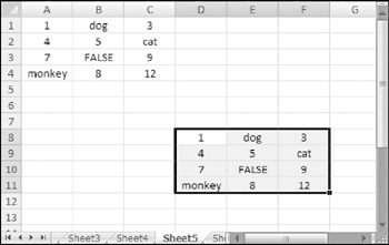 

Figure 14-7: Creating an array from a range.

The array in D8:F11 is linked to the range A1:C4. Change any value in A1:C4, and the corresponding cell in D8:F11 reflects that change.

Creating an Array Constant from Values in a Range

In the previous example, the array formula in D8:F11 essentially created a link to the cells in A1:C4. It's possible to sever this link and create an array constant made up of the values in A1:C4.

To do so, select the cells that contain the array formula (the range D8:F11, in this example). Then press F2 to edit the array formula. Press F9 to convert the cell references to values. Press Ctrl+Shift+Enter to reenter the array formula (which now uses an array constant). The array constant is as follows:

 {1,"dog",3;4,5,"cat";7,8,9;"monkey",11,12} 

Figure 14-8 shows how this looks in the formula bar.

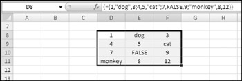
Figure 14-8: After you press F9, the formula bar displays the array constant.

Performing Operations on an Array

So far, most of the examples in this chapter simply entered arrays into ranges. The following array formula creates a rectangular array and multiplies each array element by 2:

 {={1,2,3,4;5,6,7,8;9,10,11,12}*2} 

Figure 14-9 shows the result when you enter this formula into a range.

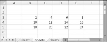
Figure 14-9: Performing a mathematical operation on an array.

The following array formula multiplies each array element by itself. Figure 14-10 shows the result when you enter this formula into a range:

 {={1,2,3,4;5,6,7,8;9,10,11,12}*{1,2,3,4;5,6,7,8;9,10,11,12}}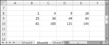 

Figure 14-10: Multiplying each array element by itself.

The following array formula is a simpler way of obtaining the same result:

 {={1,2,3,4;5,6,7,8;9,10,11,12}^2} 

If the array is stored in a range (such as A1:C4), the array formula returns the square of each value in the range, as follows:

 {=A1:C4^2} 

Tip 

In some of these examples are brackets that you must enter to define an array constant as well as brackets that Excel enters when you define an array by pressing Control+ Shift+Enter. An easy way to tell whether you must enter the brackets is to note the position of the opening curly bracket. If it's before the equal sign, Excel enters the bracket. If it's after the equal sign, you enter them.

Using Functions with an Array

As you might expect, you also can use functions with an array. The following array formula, which you can enter into a ten-cell vertical range, calculates the square root of each array element in the array constant:

 {=SQRT({1;2;3;4;5;6;7;8;9;10})} 

If the array is stored in a range, an array formula such as the one that follows returns the square root of each value in the range:

 {=SQRT(A1:A10)} 

Transposing an Array

When you transpose an array, you essentially convert rows to columns and columns to rows. In other words, you can convert a horizontal array to a vertical array and vice versa. Use Excel's TRANSPOSE function to transpose an array.

Consider the following one-dimensional horizontal array constant:

 {1,2,3,4,5} 

You can enter this array into a vertical range of cells by using the TRANSPOSE function. To do so, select a range of five cells that occupy five rows and one column. Then enter the following formula and press Ctrl+Shift+Enter:

 =TRANSPOSE({1,2,3,4,5}) 

The horizontal array is transposed, and the array elements appear in the vertical range.

Transposing a two-dimensional array works in a similar manner. Figure 14-11 shows a two- dimensional array entered into a range normally and entered into a range using the TRANSPOSE function. The formula in A1:D3 is

 {={1,2,3,4;5,6,7,8;9,10,11,12}}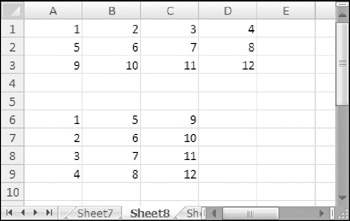 

Figure 14-11: Using the TRANSPOSE function to transpose a rectangular array.

The formula in A6:C9 is

 {=TRANSPOSE({1,2,3,4;5,6,7,8;9,10,11,12})} 

You can, of course, use the TRANSPOSE function to transpose an array stored in a range. The following formula, for example, uses an array stored in A1:C4 (four rows, three columns). You can enter this array formula into a range that consists of three rows and four columns:

 {=TRANSPOSE(A1:C4)} 

Worksheet Functions That Return an Array

Several of Excel's worksheet functions use arrays; you must enter a formula that uses one of these functions into multiple cells as an array formula. These functions are as follows: FORECAST, FREQUENCY, GROWTH, LINEST, LOGEST, MINVERSE, MMULT, and TREND. Consult the online help for more information.

Generating an Array of Consecutive Integers

As you will see in Chapter 15, it's often useful to generate an array of consecutive integers for use in an array formula. Excel's ROW function, which returns a row number, is ideal for this. Consider the array formula shown here, entered into a vertical range of 12 cells:

 {=ROW(1:12)} 

This formula generates a 12-element array that contains integers from 1 to 12. To demonstrate, select a range that consists of 12 rows and 1 column, and then enter the array formula into the range. You'll find that the range is filled with 12 consecutive integers (see Figure 14-12).

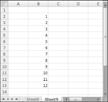
Figure 14-12: Using an array formula to generate consecutive integers.

If you want to generate an array of consecutive integers, a formula like the one shown previously is good-but not perfect. To see the problem, insert a new row above the range that contains the array formula. You'll find that Excel adjusts the row references so the array formula now reads:

 {=ROW(2:13)} 

The formula that originally generated integers from 1 to 12 now generates integers from 2 to 13.

For a better solution, use this formula:

 {=ROW(INDIRECT("1:12"))} 

This formula uses the INDIRECT function, which takes a text string as its argument. Excel does not adjust the references contained in the argument for the INDIRECT function. Therefore, this array formula always returns integers from 1 to 12.

Cross Ref 

Chapter 15 contains several examples that use the technique for generating consecutive integers.