7.6 Partitioning

---

Partitioning helps to divide an object or item into smaller chunks for easy managability and in the case of application or data it helps in easy execution or data retrieval. It works on the principle of ''divide and concur.'' Partitioning could be either an application partitioning or database partitioning. Within the database partitioning, the data could be further partitioned using some built-in features of Oracle.

7.6.1 Application partitioning

Application partitioning is defined as breaking an application into components to improve performance and effectiveness. Application partitioning could be referred to, to compose the various tiers of the enterprise system, but not including the database tier. Thus the application could be partitioned into components such as the business rules tier, web tier, persistence tier, and legacy application tier. Each partition works independently, but requires the existence of the others for their respective tasks. For example, the persistence tier is required to interface with the database when any data needs to be written to or selected from the database. The respective tiers will interface with this persistence tier and the persistence tier will communicate all requests to the database. The independent behavior of the respective tier allows for easy maintainability because each component could be upgraded or replaced independently.

Figure 7.9 illustrates a comparison using a block diagram of a partitioned and non-partitioned application. Please note that in the partitioned application the persistence layer acts as a common layer to the database. This provides a good amount of isolation of the application from the business logic, and if the database technology needs to be changed, only the persistence layer needs to be modified.

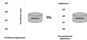
Figure 7.9: Application partitioning.

Partitioning helps in distribution of workload amongst various components and provides availability and manageability. Because each component of the application works independently, the resources utilized by each component would be what it actually needs. An example of an application that is partitioned would be an ERP system that could comprise accounts receivable, accounts payable, and payroll components. Each component works independently and communicates when it actually needs to go through some common middle layer.

7.6.2 Database partitioning

Database partitioning could be of the following:

• Physical partitioning of the database into multiple databases

• Physical distribution of data within a database into multiple partitions

Physical partitioning of the database into multiple databases takes the same principle as the application partitioning option. For example, there is a separate database for accounts payable, accounts receivable, payroll, etc. Each database acts independently. The advantage of this option is that all transactions are streamlined to a specific database based on need and usage. When this happens, other databases are idle. This helps distribution of workload amongst various databases. Another advantage of this partitioning approach is that databases that are more frequently used could be provided with additional resources.

The disadvantage of the partitioned database approach is that multiple databases have to be maintained and supported. Another disadvantage is that there cannot always be a clean boundary for accessibility between databases. Sometimes there is common data required by an application that resides in one or more databases and this adds another level of complexity because such data have to be stored in a common shareable database.

Figure 7.10 illustrates the database-partitioning scenario. Under this model each application system could be running one or more functional areas of the enterprise system. These systems are connected to one of the instances that operates against a few sets of tables which may be in separate schemas. Also note that access to certain tables by more than one component may be required, and this has to be isolated into a separate schema.

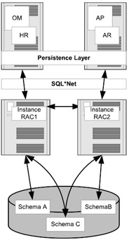
Figure 7.10: Database parti tioning.

Due to the great amount of pinging activity when data is accessed from multiple instances in an OPS environment, database partitioning provides advantages over common shared single databases. This approach helps reduce pinging because all access to a specific database or schema is done through only one node.

Under the RAC option this feature becomes redundant, because under this new architecture all transfer of data happens via the cluster interconnect and hence there is no pinging activity.

Data partitioning

Physical distribution of data within a database into multiple partitions helps the spreading of data for a table. This addresses a solution to the key problem of supporting very large tables and indexes by allowing users to decompose them into smaller and more manageable pieces called partitions, hence reducing the maintenance windows, workload distribu tion, recovery times, and impact of failures.

Workload or I/O distribution improves query performance by accessing a subset of partitions, rather than the entire table. Instead of all users' requests being funneled into one file containing all the data, they are now distributed amongst the various data files that contain this data.

Maintainability is achieved because each individual partition can exist independently, which means that if a specific partition needs to be shut down for maintenance or to perform a data restoration from backup, this would be possible. Partitioning also helps concurrent maintenance operations on different partitions on the same table or index.

Manageability is achieved because each partition of a partitioned table or index operates independently, therefore operations on one partition are not affected by the availability of other partitions. If one partition becomes unavailable because of a disk crash or administrative operation, both query and DML operations on data against other partitions are not restricted.

All operations that can be performed on regular tables can also be per formed on individual partitions of a partitioned table. For example, admin istrative activities such as rebuilding of index partitions, and backup and recovery of data partitions, could be done without affecting other partitions.

Note 

When using database partitioning the applications have to make specific connections to the respective databases, making these partitions visible to the applications. On the other hand, data partitioning of objects within a database is a physical attribute of a database and such partitioning is transparent to the application.

Partitioning of data could be done in one of several ways. Oracle provides various methods to partition data based on the business requirements, transactions, and actual physical data that are stored.

Partitioning is specified when creating the table by picking a column or set of columns to act as a partitioning key, and this key will determine which data is placed into each partition. Oracle then automatically directs DML operations to the appropriate partition based on the value of the partition key. A partition key:

• Can consist of an ordered list of 1 to 16 columns

• Can contain columns that are NULLABLE.

• Cannot contain a LEVEL, ROWID or a column of type ROWID

Note 

Partitioning is not part of the default installation; it is an add-on feature that comes bundled with the Enterprise edition of the Oracle database product.

Partitioning is useful for many different types of applications, par ticularly applications that manage large volumes of data. OLTP systems often benefit from improvements in manageability and availability, while data warehousing systems benefit from performance and manageability.

Oracle provides several partitioning methods:

1. Range partitioning

2. Hash partitioning

3. List partitioning

4. Composite partitioning

Range partitioning

Data is partitioned based on a range of column values. Each partition is defined by a value list for the partitioning keys, also referred to as the partition bound. A value list defines an open upper bound for the partition, i.e., all rows in that partition have partitioning keys that compare less than the partition bound for that partition. The partition bound for the nth partition must compare less than the partition bound for the (n + 1)th partition.

The first partition in a range partition is the partition with the lowest bound, and the last partition is the partition with the highest bound. For example, in the script below, the employee table has been partitioned by range on the employee EMPLOYEE_IDs column:

CREATE TABLE EMPLOYEE  (EMPLOYEE_ID NUMBER(6) NOT NULL  ,FIRST_NAME VARCHAR2(20)   ,LAST_NAME VARCHAR2(25) NOT NULL  ,EMAIL VARCHAR2(25) NOT NULL  ,PHONE_NUMBER VARCHAR2(20)  ,HIRE_DATE DATE NOT NULL  ,SALARY NUMBER(8,2) NOT NULL  ,COMMISSION_PCT NUMBER(2,2)  ,DEPARTMENT_ID NUMBER(4) NOT NULL  ,MANAGER_ID NUMBER(6) NOT NULL  ,JOB_ID VARCHAR2(10) NOT NULL  )  PARTITION BY RANGE (EMPLOYEE_ID)  (PARTITION EMP_DATA_P001   VALUES LESS THAN (300000)    TABLESPACE EMP_DATA_P001  , PARTITION EMP_DATA_P002   VALUES LESS THAN (600000)    TABLESPACE EMP_DATA_P002  ,PARTITION EMP_DATA_P003   VALUES LESS THAN (MAXVALUE)    TABLESPACE EMP_DATA_P003 )

In the illustration above, there are three partitions; all EMPLOYEE_IDs less than 300,000 will go into the first partition and values less than 600,000 will go into the second partition. Since that is all the anticipated immediate requirement, when the enterprise grows beyond this level any values greater than 600,000 will go to the MAXVALUE partition.

Range partitioning can also be done on two or more columns. For example, if the primary key is composed of column x and y, the range partitioning can be done on x, y. For example (EMPLOYEE_IDs, DEPARTMENT_ID):

CREATE TABLE EMPLOYEE (EMPLOYEE_ID NUMBER(6) NOT NULL ,FIRST_NAME VARCHAR2(20) ,LAST_NAME VARCHAR2(25) NOT NULL ,EMAIL VARCHAR2(25) NOT NULL ,PHONE_NUMBER VARCHAR2(20) ,HIRE_DATE DATE NOT NULL ,SALARY NUMBER(8,2) NOT NULL ,COMMISSION_PCT NUMBER(2,2) ,DEPARTMENT_ID NUMBER(4) NOT NULL ,MANAGER_ID NUMBER(6) NOT NULL ,JOB_ID VARCHAR2(10) NOT NULL ) PARTITION BY RANGE (EMPLOYEE_ID, DEPARTMENT_ID) (PARTITION EMP_DATA_P001 VALUES LESS THAN (300000,30) TABLESPACE EMP_DATA_P001 ,PARTITION EMP_DATA_P002 VALUES LESS THAN (600000,60) TABLESPACE EMP_DATA_P002 ,PARTITION EMP_DATA_P003 VALUES LESS THAN (MAXVALUE,MAXVALUE) TABLESPACE EMP_DATA_P003 )

The above script illustrates the implementation of a range partition when two or more columns are involved in determining the partitioning criteria.

Hash partitioning

Under hash partitioning, records are assigned to partitions using a hash function on values found in columns designated as the partitioning key. The main difference between the range method and hash method is that partitions of tables partitioned using the hash method have no logical meaning to the user. As a consequence, tables partitioned by hash do not support historical data, but will share all the other characteristics of range partitioning. Hash partitioning reduces adminis trative complexity by providing many of the manageability benefits of partitioning, with minimal configuration effort. The algorithm for mapping rows to tables partitioned by the hash method will aim to provide a reasonably even distribution of rows among partitions and minimize the amount of data movement.

Hash partitioning may be a better choice than range partitioning in certain situations; for example, if it is unknown how much data will map to a given range, or if the size of range partitions may differ substantially.

Due to the way that the partition mapping is implemented, it is recommended to set the number of partitions in the table to a power of 2 (2, 4, 8, 16, and so on) to avoid uneven data distribution.

Figure 7.11 illustrates how a hash partition value is distributed based on the number of partitions defined. In the figure, if the number of partitions is 5, the values are skewed; however, if the values are to the power of 2, then there is a more even distribution of values amongst the partitions.

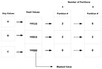
Figure 7.11: Hash partitioning mapping hash values to partitions.

The value returned by the hash routine is masked according to the number of partitions in the table. The mask takes the low-order bits necessary to satisfy the number of partitions defined. For example, two partitions will require one bit, four partitions require two, eight partitions require three, and so on. However, as shown in Figure 7.11, if the number of partitions is not a power of 2, data skewing will result because there will be some hash values that do not map to a partition. That is, five partitions will require three bits, but the values 6, 7, and 8 would not correspond to a valid partition number.

Whenever the masked value (110, 010, or 000 in Figure 7.11) is larger than the number of partitions, the low-order bits are used to determine the partition number.

When hash partitions are used, the rows are distributed among partitions in a random fashion. Adjacent rows in a given partition may have no relationship to one another. The only relationship is that their partition key hashes to the same value.

Tables partitioned using the hash method should be used:

• Where partitioning is viewed primarily as a mechanism to improve availability and manageability of large tables

• To avoid data skew between partitions

• To minimize management burden of partitioning

• Where partition pruning and partition-wise joins on a partitioning key is considered important for the database design to provide perfor mance benefits

Partition pruning is limited to equality and in-list predicates under this method.

CREATE TABLE DEPARTMENT (DEPARTMENT_ID NUMBER(4) NOT NULL ,DEPARTMENT_NAME VARCHAR2(30) NOT NULL ,LOCATION_ID NUMBER(4) NOT NULL ) PARTITION BY HASH (DEPARTMENT_ID) (PARTITION DEPT_DATA_P001 TABLESPACE DEPT_DATA_P001 ,PARTITION DEPT_DATA_P002 TABLESPACE DEPT_DATA_P002 ,PARTITION DEPT_DATA_P003 TABLESPACE DEPT_DATA_P003 ,PARTITION DEPT_DATA_P004 TABLESPACE DEPT_DATA_P004 ) /

The above script illustrates the hash partition. The department table is partitioned on DEPARTMENT_ID and is distributed into four equal partitions. Each partition will map to their respective tablespaces.

If distribution of data into various tablespaces is not a requirement and they could reside in the same tablespace, the following script should also work:

CREATE TABLE DEPARTMENT (DEPARTMENT_ID NUMBER(4) NOT NULL ,DEPARTMENT_NAME VARCHAR2(30) NOT NULL ,LOCATION_ID NUMBER(4) NOT NULL ) PARTITION BY HASH (DEPARTMENT_ID) PARTITIONS 16 /

The above script will hash partition the department table into 16 different partitions. However, system-generated partition names are assigned to these 16 partitions and the data is stored in the default tablespace of the table.

List partitioning

List partitioning is designed to allow precise control over which data belongs in each partition. For each partition, one can specify a list of possible values for the partitioning key in that partition. In a sense, one can think of this as a user-defined hash-partitioning or range-partitioning scheme.

List partitioning complements the functionality of range partitioning. Range partitioning is useful for segmenting a table along a continuous domain (most often, tables are range partitioned by ''time,'' so that each range partition contains the data for a given range of time values). In contrast, list partitioning is useful for segmenting a table along a discrete domain. Each partition in a list-partitioning scheme corresponds to a list of discrete values. An advantage of list partitioning is that unordered and unrelated sets of data can be grouped and organized in a natural way.

Tables partitioned using list method should be used if:

• The partitioning key consists of discrete data

• The user wants to group together data values that might otherwise be unrelated.

• Partition pruning and partition-wise joins on a partitioning key is considered important for the database design to provide performance benefits

CREATE TABLE LOCATION (LOCATION_ID NUMBER(4) NOT NULL ,STREET_ADDRESS VARCHAR2(40) NOT NULL ,POSTAL_CODE VARCHAR2(12) ,CITY VARCHAR2(30) NOT NULL ,STATE_CODE VARCHAR2(25) ,COUNTRY_ID VARCHAR2(2) NOT NULL ) PARTITION BY LIST (STATE_CODE) (PARTITION LOC_DATA_P001 VALUES ('MA','NY','CT','NH','ME','MD','VA','PA','NJ') TABLESPACE LOC_DATA_P001 ,PARTITION LOC_DATA_P002 VALUES ('CA,'AZ','NM','OR','WA','UT','NV','CO') TABLESPACE LOC_DATA_P002 ,PARTITION LOC_DATA_P003 VALUES ('TX','KY','TN','LA','MS','AR','AL','GA') TABLESPACE LOC_DATA_P003 ,PARTITION LOC_DATA_P004 VALUES ('OH','ND','SD','MO','IL','MI','IA') TABLESPACE LOC_DATA_P004 ,PARTITION LOC_DATA_P005 VALUES (NULL) TABLESPACE LOC_DATA_P005 ,PARTITION LOC_DATA_P006 VALUES (DEFAULT) TABLESPACE LOC_DATA_P006 ) / 

The above script illustrates the list-partitioning feature. The location table has been list partitioned on the STATE_CODE. Note that there are six partitions in all, with each partition having a list of predefined State codes. Since the State code is not mandatory and could have a null value, a separate partition has been allocated to hold all such rows. Also the last partition, which has been defined as DEFAULT, would contain any State code that has not been listed in partitions 1–4.

Composite partitioning

Composite partitioning is the result of ''composing'' range and hash or list partitioning. Under composite partitioning, a table is first partitioned using range, called the primary partition, and then each range partition is subpartitioned using the hash or list value. A subpartition of a partition has independent physical entities, which may reside in different tablespaces. Unlike range, list, and hash partitioning, with composite partitioning, subpartitions, rather than partitions, are units of backup, recovery, PDML, space management, etc. This means that a DBA could perform maintenance activities at the subpartition level.

One way of looking at a composite partition would be as a two- dimensional spreadsheet where you can have rows and columns and each row could contain the range values and the columns could contain the hash or list values.

Figure 7.12 illustrates a typical spreadsheet (two-dimensional) view of a composite partitioned table. There is a total of eight range partitions (range 1 through range 8) and each partition is subpartitioned 16 (H1 through H16) ways. Hash partitions should be divisible by 2, hence there are 16 subpartitions.

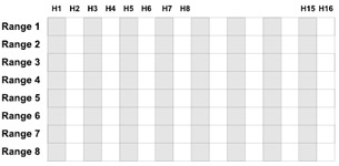
Figure 7.12: Composite partition.

Hash partitions are implicit in a composite partitioned table. Oracle does not record them in the data dictionary and hence cannot be manipulated using DDL commands. It should be noted that DDL manipulation is permitted on a range partition.

CREATE TABLE EMPLOYEE (EMPLOYEE_ID NUMBER(6) NOT NULL ,FIRST_NAME VARCHAR2(20) ,LAST_NAME VARCHAR2(25) NOT NULL ,EMAIL VARCHAR2(25) NOT NULL ,PHONE_NUMBER VARCHAR2(20) ,HIRE_DATE DATE NOT NULL ,SALARY NUMBER(8,2) NOT NULL ,COMMISSION_PCT NUMBER(2,2) ,DEPARTMENT_ID NUMBER(4) NOT NULL ,MANAGER_ID NUMBER(6) NOT NULL ,JOB_ID VARCHAR2(10) NOT NULL ) PARTITION BY RANGE (DEPARTMENT_ID) SUBPARTITION BY HASH (LAST_NAME) SUBPARTITION 8 STORE IN (EMP_DATA_HSH_P001, EMP_DATA_HSH_P002, EMP_DATA_HSH_P003, EMP_DATA_HSH_P004) (PARTITION EMP_DATA_RNG_P001 VALUES LESS THAN (30) TABLESPACE EMP_DATA_RNG_P001 ,PARTITION EMP_DATA_RNG_P002 VALUES LESS THAN (60) TABLESPACE EMP_DATA_RNG_P002 ,PARTITION EMP_DATA_RNG_P003 VALUES LESS THAN (90) TABLESPACE EMP_DATA_RNG_P003 ,PARTITION EMP_DATA_RNG_P004 VALUES LESS THAN (MAXVALUE) TABLESPACE EMP_DATA_RNG_P004 ) /

The above script illustrates the composite partitioning feature. In this script the employee table is first range partitioned on the DEPARTMENT_ID column and then hash partitioned on the LAST_NAME column. This produces a 4 by 8 matrix in place of the 8 by 16 matrix illustrated in Figure 7.12.

The records of a composite-partitioned object are assigned to partitions using a range of values found in columns designated as the partitioning key. Rows mapped to a given partition are then assigned to subpartitions of that partition using a subpartitioning method defined for the table.

Oracle 9i 

New Feature: A subpartition of the list type is a new feature in Oracle 9i. Previously in a composite partitioning option, the primary partition used to be range and the subpartition could only be hash partition.

The algorithm used to distribute rows among subpartitions of a partition, subpartitioned by hash or list, is identical to that used to distribute rows between partitions of an object partitioned by the regular hash or list partitions.

PROMPT Creating Table 'JOB_HISTORY' CREATE TABLE JOB_HISTORY (JH_ID NUMBER(10,0) NOT NULL ,END_DATE DATE NOT NULL ,START_DATE DATE NOT NULL ,EMPLOYEE_ID NUMBER(6) NOT NULL ,JOB_ID VARCHAR2(10) NOT NULL ,DEPARTMENT_ID NUMBER(4) NOT NULL ,STATE_CODE VARCHAR2(2) ) PARTITION BY RANGE (START_DATE) SUBPARTITION BY LIST (STATE_CODE) (PARTITION JH_DATA_RNG_P001 VALUES LESS THAN (TO_DATE('1-APR-2002','DD-MON-YYYY')) TABLESPACE JH_DATA_RNG_P001 (SUBPARTITION JH_DATA_LIST_P001 VALUES ('MA','NY','CT','NH','ME','MD','VA','PA', 'NJ') TABLESPACE JH_DATA_LIST_P001 ,SUBPARTITION JH_DATA_LIST_P002 VALUES ('CA,'AZ','NM','OR','WA','UT','NV','CO') TABLESPACE JH_DATA_LIST_P002 ,SUBPARTITION JH_DATA_LIST_P003 VALUES ('TX','KY','TN','LA','MS','AR','AL','GA') TABLESPACE JH_DATA_LIST_P003 ,SUBPARTITION JH_DATA_LIST_P004 VALUES('OH','ND','SD','MO','IL','MI','IA') TABLESPACE JH_DATA_LIST_P004 ,SUBPARTITION JH_DATA_LIST_P005 VALUES(NULL) TABLESPACE JH_DATA_LIST_P005 ,SUBPARTITION JH_DATA_LIST_P006 VALUES(DEFAULT) TABLESPACE JH_DATA_LIST_P006) ,PARTITION JH_DATA_RNG_P002 VALUES LESS THAN (TO_DATE('1-JUL-2002','DD-MON-YYYY')) TABLESPACE JH_DATA_RNG_P002 (SUBPARTITION JH_DATA_LIST_P007 VALUES ('MA','NY','CT','NH','ME','MD','VA','PA', 'NJ') TABLESPACE JH_DATA_LIST_P006 ,SUBPARTITION JH_DATA_LIST_P007 VALUES ('CA,'AZ','NM','OR','WA','UT','NV','CO') TABLESPACE JH_DATA_LIST_P007 ,SUBPARTITION JH_DATA_LIST_P008 VALUES ('TX','KY','TN','LA','MS','AR','AL','GA') TABLESPACE JH_DATA_LIST_P008 ,SUBPARTITION JH_DATA_LIST_P009 VALUES('OH','ND','SD','MO','IL','MI','IA') TABLESPACE JH_DATA_LIST_P009 ,SUBPARTITION JH_DATA_LIST_P010 VALUES(NULL) TABLESPACE JH_DATA_LIST_P010 ,SUBPARTITION JH_DATA_LIST_P011 VALUES(DEFAULT) TABLESPACE JH_DATA_LIST_P011) ,PARTITION JH_DATA_RNG_P003 VALUES LESS THAN (TO_DATE('1-JAN-2003','DD-MON-YYYY')) TABLESPACE JH_DATA_RNG_P003 (SUBPARTITION JH_DATA_LIST_P012 VALUES ('MA','NY','CT','NH','ME','MD','VA','PA','NJ') TABLESPACE JH_DATA_LIST_P012 ,SUBPARTITION JH_DATA_LIST_P013 VALUES ('CA,'AZ','NM','OR','WA','UT','NV','CO') TABLESPACE JH_DATA_LIST_P013 ,SUBPARTITION JH_DATA_LIST_P014 VALUES ('TX','KY','TN','LA','MS','AR','AL','GA') TABLESPACE JH_DATA_LIST_P014 ,SUBPARTITION JH_DATA_LIST_P015 VALUES ('OH','ND','SD','MO','IL','MI','IA') TABLESPACE JH_DATA_LIST_P015 ,SUBPARTITION JH_DATA_LIST_P016 VALUES (NULL) TABLESPACE JH_DATA_LIST_P016 ,SUBPARTITION JH_DATA_LIST_P017 VALUES (DEFAULT) TABLESPACE JH_DATA_LIST_P017) ) / 

The above script illustrates a composite partitioning features. In this script the JOB_HISTORY table is first range partitioned on date and then subpartitioned using the list partitioning feature on STATE_CODE.

Objects partitioned using the composite method have logical meaning (defined by their partition bounds) but have no physical presence (since all data mapped into a partition resides in segments of subpartitions associated with it). Subpartitions have no logical meaning beyond the partition to which they belong. As a consequence, objects partitioned using the composite method:

• Support historical data (at partition level)

• Support use of subpartitions as units of parallelism (for PDML), space management, backup, and recovery

• Are subject to partition pruning and partition-wise join on the range, list and hash dimensions

• Support parallel index access

Note 

The number of hash partitions or composite partitions, subparti tioned by hash values should be a power of 2 (2, 4, 8, 16, ...).

Partitioned indexes

Data contained in tables can be partitioned, but what about the corresponding indexes? Yes, the index can also be partitioned. Similar to a data partition, index partitioning will help improve manageability, availability, performance, and scalability. Partitioning of indexes can be done in one of two ways, either independent of the data partition, where the index is of a global nature (global indexes) or dependent on the data partition by directly linking to the partitioning method of tables where the indexing is of a local nature (local indexes).

Local indexes

Each partition in a local index is associated exactly with one partition of the table. This enables Oracle to automatically keep the index partitions in sync with the table partitions. Any actions performed by the DBA on one partition, like rebuilding of a partition, reorganization of a partition, etc., only affect that single partition.

Global indexes

Global indexes are opposite to the locally partitioned indexes, in that a global index is associated with more than one partition of the table. The global index by itself could be either partitioned or non-partitioned. In an OLTP environment where a table has multiple indexes to help in query performance, these indexes are normally created as a non- partitioned global index. Under these circumstances, a local index may not provide benefits that a global non-partitioned index would provide, because of the manner in which the rows are distributed.

Global indexes are normally created on columns with duplicate values and these values could be present in any of the underlying data partitions. In these situations a local index would not be feasible because there is no one-to-one mapping between the data partition and the index. When a query needs to determine a row in a global index, it will help identify the row and the corresponding table partition that it belongs in.

7.6.3 Benefits of partitioning

Partitioning provides great benefits to performance in either a single instance environment or a RAC environment. However, compared to a non-partitioned implementation, a partitioned implementation is definitely a better option in a RAC environment. When multiple users access the data from multiple instances, there is no guarantee that users will be accessing data that reside in different partitions; also there is no guarantee that users will be accessing data from the same partitions. However, under situations where users do not access the same data, Oracle will have less lock information to be shared across the cluster interconnect. This is because when users access different partitions, the lock that is placed at the partition is unique to the instance from which the user has accessed the row, hence there is less sharing of lock information across the cluster interconnect.

Apart from the interinstance locking benefits available to a RAC implementation, partitioning provides the following general performance benefits that are common to both a single instance configuration and a parallel instance configuration:

• Partition independence

• Partition pruning

• Partition-wise joins

• Parallel DML

Partition independence

This partitioning feature provides a great amount of flexibility for the DBA. Often, there are maintenance activities like tablespace reorganiza tion, rebuilding of indexes, recovery of data pertaining to a table, etc., that require that the entire database be shut down so that these tasks can be completed. This affects the businesses directly due to interrupted services, and if there is an SLA, this adds to the problem.

With partitioning, only certain partitions need to be shut down for maintenance. This means that only users accessing data from a specific partition will be affected. For example, in an organization that supports many companies (very common in today's Internet-based business), if the data is partitioned based on company, then if a partition is not available only certain companies that belong to that partition are affected. This also allows for scheduled maintenance. The DBA group could inform the appropriate companies of scheduled outages or, if the database only supported one organization and the data was partitioned by region (eastern, western, etc.), outages may be scheduled based on regional activity. This is common in banking applications, where for certain periods of time during the day, customers belonging to a specific region are not allowed access to the data when maintenance is being performed.

Partition pruning

This is one of the most effective and intuitive ways in which partitioning improves performance. Based on the queries optimization plan, it can eliminate one or more unnecessary partitions or subpartitions from the queries execution plan, focusing directly on the partition or subpartition where the data resides.

For example, if the optimizer determines that the selection criteria used for pruning are satisfied by all the rows in the accessed partition or subpartition, it removes those criteria from the predicate list (WHERE clause) during evaluation in order to improve performance. However, there are certain limitations on using certain features; the optimizer cannot prune partitions if the SQL statement applies a function to the partitioning column. Similarly, the optimizer cannot use an index if the SQL statement applies a function to the indexed column, unless it is a function-based index.

Partition pruning occurs when there is an appropriate predicate on the partitioning key of a partitioned table. For range and list partitioning, partition pruning occurs for both equality and inequality predicates. In hash partitioning, partition pruning will occur only for equality predicates.

Note 

Partitioning works best with the cost-based optimizer and when the statistics have been collected. This helps Oracle identify and create the best execution plan to get to the right partition that contains the rows.

Partition-wise joins

Another performance benefit of partitioning is partition-wise joins. The performance enhancement is effective for joining tables that are partitioned identically on the join keys (equipartitioned). By recognizing that two tables are equipartitioned, Oracle optimizer will consider new join methods that leverage these partitioning characteristics.

A partition-wise join is a join optimization that you can use when joining two tables that are both partitioned along the join column(s). Partition-wise joins occur when two or more tables and/or indexes are equipartitioned and joined using the partition columns. That is, if the tables and/or indexes have the same partition columns, same number of partitions, and the same range values for range partitions, then the optimizer is able to perform joins partition by partition. By working with smaller sets, the number of rows that need to be joined is smaller, resulting in faster processing.

With partition-wise joins, the join operation is broken into smaller joins that are performed sequentially or in parallel. Another way of looking at partition-wise joins is that they minimize the amount of data exchanged among parallel slaves during the execution of parallel joins by taking into account data distribution.

Figure 7.13 illustrates a comparison with the traditional partition join operation where all the tables of the entire database are joined to complete the operation. However, with the partition-wise join, many smaller partition join operations are performed.

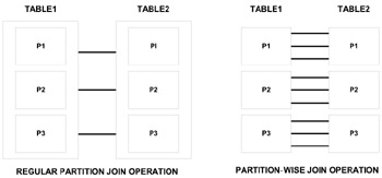
Figure 7.13: Regular full partition join vs. partition-wise join operation.

A partition-wise join divides a large join into smaller joins between a pair of partitions from the two joined tables. To use this feature, you must equipartition both tables on their join keys. For example, consider a large join between a SALES table and a PRODUCT table on the column PRODUCT_ID. The following is an example of this:

SELECT     PRODUCT_NAME,      COUNT(*) FROM SALES, PRODUCT WHERE PRODUCT.PRODUCT_ID = SALES.PRODUCT_ID AND SALES.SALES_DATE BETWEEN TO_DATE(01-JUN-2002, DD-MON-YYYY) AND TO_DATE(01-DEC-2002, DD-MON-YYYY) GROUP BY PRODUCT.PRODUCT_NAME HAVING COUNT(*) > 1000;

This is a very large join typical in data warehousing environments. The entire PRODUCT table is joined with one-quarter of the SALES data. In large data warehouse applications, it might mean joining millions of rows. The join method to use in that case is obviously a hash join. But you can reduce the processing time for these hash joins even more if both tables are equipartitioned on the PRODUCT_ID column. This enables a full partition- wise join.

Partition-wise joins are specifically useful in a RAC environment because they reduce join-processing time and significantly reduce the volume of interconnect traffic amongst the participating instances. Another major benefit in using this feature is that it requires less memory compared to the traditional join operation, where the complete data set of the tables is joined.

Partition-wise joins could be full joins or partial joins. The advantages of partition-wise joins are more visible when used against the composite partitions.

Parallel DML

Parallel execution dramatically reduces response time for data-intensive operations on large databases typically associated with decision support systems (DSS) and data warehouses. In addition to conventional tables, parallel query and PDML can be used with range and hash-partitioned tables. This enhances scalability and performance for batch operations.

7.6.4 Partition maintenance

Like any other DDL operations that are available for maintaining the metadata, partitioning is just another feature and has a similar set of DDL operations that a DBA could apply for regular maintenance on the various partitioning methods.

While we can create a partition, we can also drop, modify, exchange, add, move, and split partitions.

Note 

Unless otherwise mentioned, the options below are available for all the partitioning methods.

Split partition

As the name suggests, the SPLIT PARTITION command will split an existing partition into two or more partitions. The current set of data is moved from the existing partition into the new partition based on the partitioning values or ranges. A list or range partition could be split into two or more values:

ALTER TABLE <> SPLIT PARTITION <>   VALUES ( ) INTO (PARTITION <>, PARTITION <>);

The EMPLOYEE table used in the previous discussion on range partitions consisted of three partitions:

PARTITION BY RANGE (EMPLOYEE_ID) (PARTITION EMP_DATA_P001 VALUES LESS THAN (300000) TABLESPACE EMP_DATA_P001 , PARTITION EMP_DATA_P002 VALUES LESS THAN (600000) TABLESPACE EMP_DATA_P002 , PARTITION EMP_DATA_P003 VALUES LESS THAN (MAXVALUE) TABLESPACE EMP_DATA_P003 )

As the use grows, new employees are added and the MAXVALUE partition becomes so dense that it needs to be repartitioned. Using Oracle's split partitioning feature the MAXVALUE partition could be split into one range partition of 900000 and another continuing to be the new MAXVALUE partition.

ALTER TABLE EMPLOYEE SPLIT PARTITION PK_EMPLOYEE AT (900000) INTO ( PARTITION EMP_DATE_P003 VALUES LESS THAN (900000) TABLESPACE EMP_DATA_P003 , PARTITION EMP_DATA_P004 VALUES LESS THAN (MAXVALUE) TABLESPACE EMP_DATA_P004 ) 

Note 

After a SPLIT PARTITION has been performed, the underlying indexes have to be rebuilt to reflect this new partitioning structure.

Merge partition

Again, as the name suggests, the MERGE PARTITION command combines two or more existing partitions into one. However, only two adjacent partitions can be combined:

ALTER TABLE <> MERGE PARTITION <>.<>, INTO PARTITION <>;

The EMPLOYEE table used in the previous discussion under SPLIT PARTITION consisted of four partitions (after the split):

PARTITION BY RANGE (EMPLOYEE_ID) (PARTITION EMP_DATA_P001 VALUES LESS THAN (300000) TABLESPACE EMP_DATA_P001 , PARTITION EMP_DATA_P002 VALUES LESS THAN (600000) TABLESPACE EMP_DATA_P002 , PARTITION EMP_DATA_P003 VALUES LESS THAN (900000) TABLESPACE EMP_DATA_P003 , PARTITION EMP_DATA_P004 VALUES LESS THAN (MAXVALUE) TABLESPACE EMP_DATE_P004 )

After a few years when many employees leave and new employees join the partition, EMP_DATA_P002 may have so few employees that a separate partition may not required to be maintained. In such circumstances the EMP_DATA_P002 and EMP_DATA_P003 could be merged to form one partition.

ALTER TABLE EMPLOYEE MERGE PARTITION EMP_DATA_P002, EMP_DATA_P003 INTO PARTITION EMP_DATA_P003

Note 

After a MERGE PARTITION has been performed, the underlying indexes have to be rebuilt to reflect this new partitioning structure.

Drop, truncate, or exchange partition

The DROP PARTITION, TRUNCATE PARTITION,or EXCHANGE PARTITION command removes an existing partition. When a partition that is in the middle is dropped, any future data that belongs to the dropped partition will be inserted into the next available partition. When a partition is dropped, the data is also dropped. This operation works exactly the same in all the partitioning methods.

TRUNCATE PARTITION is similar to DROP PARTITION. However, with TRUNCATE PARTITION, all rows are removed from the table partition. If the partition being truncated has a LOCAL index, truncating the table partition will also truncate the corresponding local index partition.

Table definitions could be changed from a non-partitioned to a partitioned structure or from a partitioned to a non-partitioned structure by exchanging their data segments. This feature is useful when migrating from a non-partitioned table structure to a partitioned table structure.

Move partition

The MOVE PARTITION command moves the data from the current partition to another partition. If data in an existing partition is being dropped or truncated, and the data is required, the data could be combined into another partition either using the MERGE PARTITION option or MOVE PARTITION option.

One of the key features of Oracle that would help in meeting the requirements of high volume, high availability, and highly scalable systems is the partitioning option. As discussed, this feature provides a wealth of benefits in performance and distribution of data in a RAC implementation. It would be in the best interest of the enterprise to implement the database with a data-partitioning feature, especially for tables that have a large number of rows.

While data could be distributed into partitions, it must be stored permanently on disk using a storage mechanism. In Chapter 2 (Hardware Concepts) we discussed some of the benefits of the various storage subsystems. There is a layer above the physical storage subsystem and the partition, the tablespace. The tablespace that contains the partition could be managed either using the data dictionary, which is the default, or could be maintained using a bitmap structure at the header using LMT.

---