7.4 Selecting the right indexing method

---

Oracle provides various indexing methods that could be utilized based on the data or column being indexed and the access patterns on the columns. Selecting the right indexing strategy also depends on various factors, type of data being stored, uniqueness of data, cardinality of data, etc.

We have in the previous section looked into indexing options used in a partitioned table, namely local indexes and global indexes. While these are just types of indexes, they could be implemented using various indexing methods, for example, bitmap indexes and B-tree indexes. So the challenge is not in the selection of the type of index, which is easier because it goes one-on-one with the type of implementation (e.g., partitioned indexes) but in the selection of the method used in indexing the tables. The various indexing methods are:

• B-Tree indexes

• Reverse key indexes

• Compressed indexes

• Bitmap indexes

• Bitmap join indexes

• Index organized tables

• Function-based indexes

7.4.1 B-tree indexes

This is the default type of index, i.e., if an index type is not mentioned during the creation of an index, this is the type of index that is created. A B-tree index is a binary tree structure that has branches and leaf nodes. When data is to be retrieved, Oracle will, starting at the root block, step through the branches and leaf blocks to arrive at the correct row that contains the matching data.

A structure of a B-tree index is illustrated in Figure 7.3. From the figure it should be noted that Oracle does not create many tiers of branches and leaf blocks. Initially each index tree has one level. If the data in the table is very small, there may be only one index block. In that case, the leaf block is the same as the branch block. As the data grows, the level increases and then there is a branch block and a leaf block with a parent–child relationship. The maximum number of levels that the B-tree index can grow to is 24 (i.e., 0 to 23), which means that with two rows per index block it can hold approximately 18 billion leaf blocks.

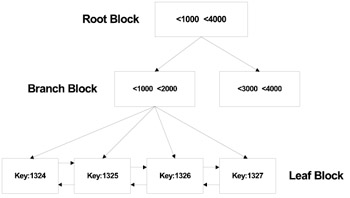
Figure 7.3: B-tree index.

The root block contains data that points to the branch block, which in turn points to the lower level leaf block. The lowest level contains the indexed data values and corresponding ROWIDs required for locating the row.

Figure 7.4 illustrates the B-tree index leaf block structure. Various index types carry different structures. The B-tree structure has the following advantages:

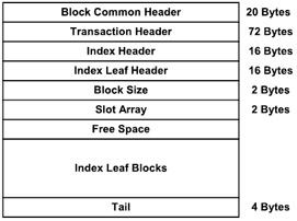
Figure 7.4: B-tree index leaf block structure.

• All leaf blocks of the tree are at the same depth, so retrieval of any record from anywhere in the index takes approximately the same amount of time. It is important that the index tree does not get very shallow, and hence a tree structure that is more than four levels deep would be inefficient.

• B-tree indexes automatically stay balanced.

• All blocks of the B-tree are three-quarters full on the average.

• B-trees provide excellent retrieval performance for a wide range of queries, including exact match and range searches.

Figure 7.5 illustrates a dissection of the index block. This level of detail is obtained by taking a dump of the index header.

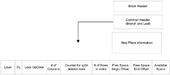
Figure 7.5: B-tree index block layout.

The number of blocks that Oracle has to read before it reaches the actual leaf block is normally low, and depends on the Oracle default block size defined during the database creation.

Note 

In the case where a multiblock database is created using Oracle 9i, unless specified at the tablespace level, the default block size applies to the number of blocks read by Oracle.

The leaf blocks are created based on the permutation of values that are present during the initial creation of index and subsequent inserts. When a specific index leaf block is filled, another block is allocated by Oracle from the FREELIST (not applicable in the case of locally managed tablespaces). If the index key value falls between the existing keys, Oracle performs an index leaf block split, which means that the upper half of the keys is transferred to the new block while the lower half remains in the old or existing block.

B-tree indexes provide considerable performance benefits where the index key value is unique across the database. Performance degradation of the B-tree index can be noticed when the index key value is non-unique and the number of rows per value gets higher.

B-tree indexes are useful in a RAC environment provided there is no collision of index key values and the inserts into the leaf blocks are not adjacent to each other. If the values being inserted are sequential in nature, which means they are most likely to be inserted into the same leaf block, performance degradation occurs due to frequent index leaf block splits. Under such situations it would be advisable to use the reverse key index option.

7.4.2 Reverse key indexes

A reverse key index reverses the bytes of each column value indexed while keeping the column order. By reversing the keys of the index, the insertions become distributed across all leaf keys in the index. A reverse key index can be used in situations in which the user inserts ascending values and deletes lower values from the table, such as when using sequence-generated (surrogate keys) primary keys.

When using a surrogate key, especially in an insert-intensive application, the lowest level index leaf block will encounter extensive contention. In Figure 7.3 above, the key values 1324, 1325, 1326, etc., are sequentially written in ascending order. This would require a change to the leaf block, and when rows are inserted concurrently it causes block splits to happen more frequently. The end result is a potential performance bottleneck. This overhead is even more significant in the OPS/RAC environment where multiple users insert data from different Oracle instances.

As the word REVERSE implies, the actual key value is reversed before being inserted into the index. For example, if the value of 4567 was reversed its new value would be 7654. We will now see how this works.

When numbers are sequentially generated in ascending order, this has a significant effect in the distribution and scalability for an insert-intensive application. With the reverse option specified with the index creation statement, the potential issues described in Figure 7.3 could be avoided. REVERSE key indexes are created using the following command:

CREATE INDEX PK_JBHIST ON JOB_HISTORY (JOBHIST_ID) REVERSE;

Table 7.1 illustrates the corresponding reverse key values to the natural key/surrogate key shown in Figure 7.3.

Table 7.1: Natural and Reverse Key Values

Natural Key	Reverse Key
1234	4321
1235	5321
1236	6321
1237	7321

The following questions become inevitable:

1. What does this do to accessibility?

2. Do we have to change code to reflect the reverse structure?

The answer is that there are absolutely no effects on accessibility and there is no need to change the code. This is due to the fact that the reverse structure is maintained at the index segment level and is not visible to the application or user.

This is true even when the partitioned options of the database are used, the same rule applies; the index segment is reversed individually rather than the index being reversed and then partitioned. The ROWID is not changed and neither is the column order.

When the REVERSE option is used during index creation, the B-tree index structure at the leaf block level is illustrated in Figure 7.6. (For easy comparison, the example from Figure 7.3 has been used.) Figure 7.6 represents the reverse key structure (the natural key values in this example should be the reverse of what is shown in the leaf blocks.) It is noticeable that the keys are distributed and will help the indexes to scale.

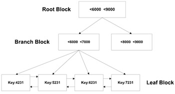
Figure 7.6: Reverse key index leaf block structure.

In an OPS/RAC configuration, when an index is based on a column that uses a surrogate key, and two or more instances are inserting data, there is a strong likelihood that both instances will be contending for the same index block. This is because sequential index entries are likely to be in the same block. Reverse key indexes reverse the bytes in each index entry, causing sequential entries to be dispersed and distributed across the index leaf block. This causes reduced contention at the index block. When it comes to performance of insert-intensive applications, the transactions per second (TPS) increase when the reverse option is used on a surrogate key using B-tree indexes, which in turn improves the performance.

In the case of concatenated indexes, the reverse keys feature will also provide similar benefits. This is because the reverse operation is performed individually on each column before they are concatenated. For example, if the model in Figure 7.1 above is implemented and if there exists a concatenated index in the JOB_HISTORY table between the JOBHIST_ID and EMP_ID, the concatenated index when the REVERSE option is implemented would be REVERSE (JOBHIST_ID) | REVERSE (EMP_ID) instead of REVERSE (JOBHIST_ID j EMP_ID).

Note 

While this is an excellent choice for OLTP applications where the queries are mostly singleton select and the insert operations are intensive, it is bad for DSS, reporting, and data warehouse applications.

In a DSS or a data warehouse application, queries are not singleton selects but rather retrieval of large numbers of rows requiring a range of data. In Figure 7.6 above, the surrogate keys that have the original values of 1324, 1325, 1325, etc., are in multiple leaf blocks rather than together. When queries make range retrieval, they would have to scan multiple dispersed blocks rather than adjacent blocks. This causes significant performance problems in a DSS or data warehouse application.

When using a reverse key clause, an index block typically references more rows than that contained in each data block for the corresponding table. One major factor for this is the density of the leaf blocks. Unlike a normal B-tree index leaf block, these blocks do not reach 100% density due to the distributed structure.

7.4.3 Compressed indexes

Compressed indexes compress portions of the primary key column values in an index or index-organized table, which reduces the storage overhead of repeated values. Keys in an index comprise two pieces, the grouping piece and a unique piece. If the key is not defined to have a unique piece, Oracle provides one in the form of a row appended to the grouping piece; these pieces are called prefix and suffix, respectively. Oracle provides compression by sharing the prefix among the suffix entries in an index block, while compressing only the leaf level blocks of the B-tree index. In the branch blocks the key suffix can be truncated; however, the key is not compressed.

Compressed indexes provide both storage and performance advantages. Compression of the leaf blocks provides a huge saving in space, which allows more keys in each index block, which can lead to less I/O and better performance. However, because the key columns are reconstructed every time during an index scan, there could potentially be additional CPU consumption.

Figure 7.7 represents the index leaf block structure for a compressed B-tree index. Please note that compared to the regular B-tree index, the compressed B-tree index block has more parts and takes more space for the block level information. The structure has additional block level information such as the compression header, and suffix and prefix slots, which are not found in the regular B-tree index.

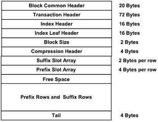
Figure 7.7: B-tree index compressed leaf block structure.

7.4.4 Bitmap indexes

Bitmap indexes were first introduced in Oracle Version 7.3 and were probably the first type of index outside the traditional B-tree index.

The B-tree indexes are commonly used in an OLTP application where the uniqueness of the key value can be maintained to a great extent. When the uniqueness of the key value changes, or where a value in a column is repeated hundreds or thousands of times, performance of the query to retrieve rows using a B-tree index would be significantly poor. A bitmap index would be ideal in such situations. A bitmap index is typically less than 25% of the size of a regular B-tree index and can be scanned very quickly.

Due to the support for columns with large numbers of duplicate values, a bitmap index is suited for a data warehousing application and is not appropriate for an OLTP application.

The bitmap is compressed before it is stored in the index. If a value in the bitmap changes, then the compressed bitmap must first be uncompressed. After the bits are changed in the bitmap, the bitmap is again compressed for storage in the index. This is another reason why bitmap indexes are suitable in a data warehouse application, because here the data values are seldom modified, and hence such an application does not have this additional overhead.

It should be noted that updates to a table covered by a bitmap index are deferred until the entire DML operation is complete. This means that irrespective of the number of rows being modified, the bitmap will not be updated until the end of the entire operation.

Bitmap indexes are a perfect choice for a data warehouse application implemented on a stand-alone configuration or a RAC implementation.

7.4.5 Bitmap join indexes

A ''join index'' is an index structure that spans multiple tables and improves the performance of joins of those tables. Bitmap join indexes provide improved performance benefits for a specific class of join queries, namely star queries used in data warehouse schemas.

In the previous section we stated that in a regular bitmap index, each distinct value for the specified column is associated with a bitmap where each bit represents a row in the table. Bitmap join indexes extend this concept such that the index contains the data to support the join query, allowing the query to retrieve the data from the index rather than referencing the join tables.

A bitmap join index uses a compressed storage mechanism to store the join index values, and hence requires less storage space.

Suppose that a data warehouse contains a star schema with a fact table named SALES and a dimension table named PRODUCT, which holds each product brand. A bitmap join index can be created which indexes sales by product brands. Here is the SQL for the index:

CREATE BITMAP INDEX PROD_SALES_BJI ON SALES (PRODUCT.BRAND) FROM SALES, PRODUCT WHERE SALES.PRODUCT_ID = PRODUCT.PRODUCT_ID 

The bitmap join index above could be used to evaluate the following query. In this query, the PRODUCT table will not even be accessed; the query is executed using only the bitmap join index and the sales table.

SELECT SUM (SALES.AMOUNT) FROM SALES, PRODUCT WHERE SALES.PRODUCT_ID  = PRODUCT.PRODUCT_ID AND PRODUCT.BRAND  = 'KELLOGS'

If the PRODUCT table is large (and product-based dimension tables can reach tens of millions of records), then the bitmap join index can vastly improve performance by not requiring any access to the PRODUCT table. In addition, bitmap join indexes can eliminate some of the key iteration and bitmap merge work, which is often present in star queries with bitmap indexes on the fact table.

Oracle 9i 

New Feature: The bitmap join index is a new type of index introduced in Oracle 9i. This feature is specifically useful for data warehouse operations involving star queries.

7.4.6 Index-organized tables

Index-organized tables (IOT) store data in B-tree structures similar to the indexes on a regular table. However, these tables minimize overall storage requirement, because the index and the data are stored together and do not require additional storage for the index structures. Another major difference between a regular B-tree index and an IOT is that in a regular B-tree, Oracle maps the index to the corresponding row through a ROWID value. IOTs do not have a ROWID.

In an IOT, the B-tree entries at the leaf block level are very large because they consist of both the key and non-key column values. If the index entry gets very large, then the leaf node may end up storing more finite row information, thereby destroying the dense property of the B-tree index.

Figure 7.8 illustrates the leaf block structure of an index-organized table. Please note that while the root and branch blocks are similar to a regular B-tree index, the leaf blocks are different

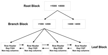
Figure 7.8: IOT leaf block structure.

Applications that could potential benefit from using an IOT are:

• Information retrieval applications

• Spatial applications

• OLAP applications

IOT supports secondary indexes on columns that are neither the primary key nor a prefix of the primary key. These secondary indexes are created using logical row identifiers. Each logical row used in a secondary index is based on the table's primary key and can also include a physical guess, which identifies the block location of the row in the IOT at the time when the secondary index was created or rebuilt.

Logical ROWIDs give the fastest possible access to rows in IOTs by using two methods:

• The physical guess whose access time is equal to that of physical ROWIDs

• Access without the guess (incorrect guess), which performs like a primary key access of the IOT

The guess is based on knowledge of the file and block that a row resides in. If the guess is wrong and the row no longer resides in the specified block, then the remaining portion of the ROWID, the primary key, is used to get the row. Thus if the guess is right, only one block read is required, making performance comparable to that of physical ROWIDs.

7.4.7 Function-based indexes

Most of the time in a query operation, a function or two is used to qualify criteria to retrieve the row. These operations cause full table scans on tables referenced in the query. On large tables such operations cause performance bottlenecks. A function-based index computes the value of the function or expression and stores it in the index. So when a query that contains the function is executed, it directly takes benefit of the stored functional values and makes a quick data retrieval.

Function-based indexes can be created to materialize computational intensive expression in the index, so that the server would not need to compute the value of the expression when processing SELECT and DML statements. For example:

CREATE INDEX SALES_MARGIN_INDX ON SALES (REVENUE-COST);

---