Time Stamps, Waveforms, and Dynamic Data

Often, data that you want to analyze or acquire is a function of time. For example, we might be interested in seeing how temperature varies over the time of day, or how vibrational waveforms look when plotted over a time axis.

LabVIEW has some special data types that make it easier for the casual user to analyze and present this type of data in plots. These are the time stamp, waveform, and dynamic data. Time stamps are used to store the timing information in waveforms and multiple waveforms can be stored in dynamic data. Because there is a natural dependency from time stamp to waveform to dynamic data, we will introduce these topics in this order.

Time Stamp

The time stamp is a data type that stores an absolute date/time value, such as the time of a data collection event, with very high precision (19 digits of precision each in both the whole second and fractions of a second).

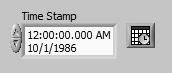
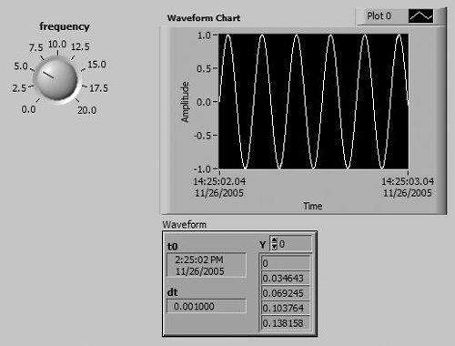
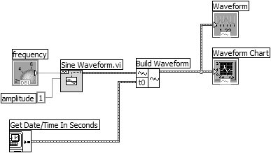
A numeric control can also be used to store and display time stamp values (we can change the display format to date/time), but the numeric control holds only a relative quantity. The time stamp control holds an absolute quantity.

In the previous activity, we used the Get Date/Time In Seconds function to obtain a time stamp of the current time (see Figure 8.59), which was used to set the t0 (initial time) of the sine waveform. The waveform data type uses a time stamp to store its t0 value.

Figure 8.59. Time Stamp control

The time stamp is not only a highly precise way of storing absolute time information; the time stamp control (shown in Figure 8.59) is very useful for viewing and editing time stamp values. The time stamp control may be found in the Modern>>Numeric subpalette of the Controls palette.

You can edit the time stamp value by clicking on the portion of time you wish to change and then using the up arrow and down arrow keys to increment and decrement the value. Or you can use your keyboard to type a value to replace the selected value. You can also pop up on the time stamp control and select Data Operations>>Set Time to Now to set the time stamp value to the current date and time.

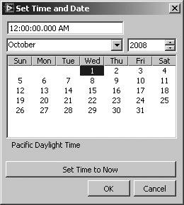
Date/Time Browse Button

But, there is another way to edit the time stamp that is a lot more fun. Click the Time/Date Browse button to display the Set Time and Date dialog box, shown in Figure 8.60. From this dialog, you can easily edit the date and time value of the time stamp using a calendar-like interface.

Figure 8.60. Set Time and Date dialog

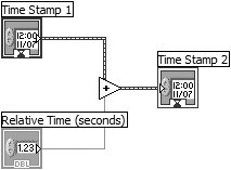
You can also right-click time stamp controls, indicators, and constants and select Data Operations>>Set Time and Date from the shortcut menu to display the Set Time and Date dialog box. This is especially useful for time stamp constants and indicators, which do not have a Time/Date Browse button.

Relative Time Calculations

Often you will want to perform time calculations. For example, the code shown in Figure 8.61 shows how to calculate the relative time between two time stamps using the Subtract function.

Figure 8.61. Calculating relative time by subtracting time stamps

For example, you can use this technique to build a performance benchmarking template, such as the one shown in Figure 8.62. Simply capture time stamps in the first and last frames of a Flat Sequence Structure and subtract the end time from the start time to yield the total execution time of your code in the middle frame. This is an excellent demonstration of how you can use a Flat Sequence Structure for application timing and synchronization tasks.

Figure 8.62. Performance benchmarking template that calculates the time required to execute the code in the center frame of a Flat Sequence Structure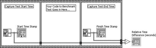

The operation of adding relative time to a time stamp can be done with the Add function, as shown in Figure 8.63.

Figure 8.63. Adding relative time to a time stamp

Time Stamp and Numeric Conversion

As you see in Figures 8.62 and Figure 8.63, the time stamp and numeric data types are closely related, and there are instances where you will need to convert between the two. Functions such as Add and Subtract will either adapt (because they are polymorphic) to a time stamp or coerce it to a DBL. But, sometimes you will want to explicitly perform this conversion. Use the To Double Precision Float function (available from the Programming>>Numeric>>Conversion palette) to convert a time stamp to a DBL (see Figure 8.64). Use To Time Stamp (also available from the Programming>>Numeric>>Conversion palette, but more easily available from the Programming>>Timing palette) to convert a numeric to a time stamp (see Figure 8.65).

Figure 8.64. To Double Precision Float

Figure 8.65. To Time Stamp

The To Double Precision Float function (shown in Figure 8.64) will convert any numeric to a DBL. It also works for converting a time stamp to a DBL, which is a sometimes overlooked (but extremely useful) fact.

Waveforms

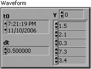
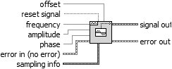
In many engineering and scientific applications, much of data you handle is a collection of values that vary over time. For example, audio signals are pressure values versus time; an EKG is voltage versus time; the variations in the surface of a liquid as a pebble drops in are x,y,z coordinates versus time; the digital signals used by computers are binary patterns versus time. LabVIEW provides you with a convenient way to organize and work with this kind of time-varying datathe waveform data type. A waveform data type allows you to store not only the main values of your data, but also the time stamp of when the first point was collected, the time delay between each data point, and notes about the data. It is similar to other LabVIEW dataypes like arrays and clusters; you can add, subtract, and perform many other operations directly on the waveforms. You can create Waveform and Digital Waveform controls on the front panel from the I/O palette (see Figure 8.66 and Figure 8.68). The corresponding block diagram representations are brown/orange for waveform terminal and green for the digital waveform terminal (see Figure 8.67 and Figure 8.69).

Figure 8.66. Waveform control

Figure 8.67. Waveform terminal

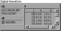
The analog waveform was introduced in LabVIEW prior to the introduction of the digital waveform, and it was simply called a "waveform." Thus, LabVIEW will still occasionally use "waveform" when referring to analog waveforms. In this book, we will try to use "analog waveform" and "digital waveform," but when referring to LabVIEW features, we will use the names used by LabVIEW. For example LabVIEW refers to the analog waveform control as "waveform" and the digital waveform control as "digital waveform."

Figure 8.68. Digital Waveform control

Figure 8.69. Digital Waveform terminal

Analog Waveform Symbol

LabVIEW uses different symbols for analog and digital waveforms, as you can see on the terminals shown here. The analog waveform symbol looks like a small sine wave and the digital waveform symbol looks like a small square wave. You will see these same symbols on waveform functions, VI icons, and elsewhere. So keep a sharp eye out for themthey will help you identify which waveform data type you are working with.

Digital Waveform Symbol

Also, the color of the analog waveform type is brown with orange (the colors of clusters and floating points), while the color of the digital waveform type is green (the color of Booleans). The wire pattern of all waveforms is the same as that of the cluster.

Examining the waveform data type a little more closely, we see it is really just a special type of cluster that consists of four components, called Y, t0, dt, and Attributes:

Y: This component is the data that varies with time. For an analog waveform, this is a 1-D array of numeric data points, which can be either a single point or another waveform, depending on the operation. The representation of the analog 1-D array is DBL. Discrete signals (signals that usually only have two states, such as true or false, 0 or 5V, on or off, etc.) are called "digital" signals. For these, we use a digital waveform. For a digital waveform, the Y component is digital data, which is another special data type that we will discuss shortlyfor now you can think of it as a table of binary values where the columns are the digital lines and the rows are the successive valuesbasically, a 1-D array of port states (a port is a group of digital lines).
t0: This component is a time stamp value that represents the time (according to the system clock) when the first point in the Y array was acquired. It is also referred to as the initial time or the time stamp. We learned about the time stamp data type in the previous section.
dt: Δt, or delta-t, is a scalar value that represents the time between data points in the Y array.
Attribute: By default, this component is hidden (you can see it by popping up and selecting Visible Items>>Attribute). Attributes, which are always optional, are variant data types that conveniently allow you to bundle custom information (as named attributes of the variant) along with your waveform such as the device number or channel number of your data acquisition system. Attributes do not affect how the data looks or its Y or time values. Variants are a very flexible data type that will accept any other LabVIEW data typewe will learn more about them in Chapter 12.

In Figure 8.66, the waveform control shows that the first point of the waveform starts at 07:21:19 PM, on Nov. 10, 2006, and that the time between each point is 0.5 seconds.

Waveforms Versus Arrays

In many ways, you can think of waveforms as just 1-D arrays that hold your datawith some extra information attached about the time and timing of the data points. Waveforms are most often useful in analog data acquisition, which we'll discuss in Chapter 10, "Signal Measurement and Generation: Data Acquisition," and Chapter 11, "Data Acquisition in LabVIEW."

Of course, you do not necessarily need to use waveform data types; you can always just use arrays to hold your data. However, waveform data types offer several advantages over arrays:

The presence of t0. Without t0, you would not know when your data were taken. The waveform data type automatically returns the time of day and the date in the t0 component, which gives you a real-world acquisition time for your data.
Easier Graphing. The waveform data type also simplifies graphing your data. In previous versions of LabVIEW, you had to bundle the value of the initial point (x0) and the time between points (delta x) with your data (Y array). The waveform data type already contains these elements, so all you have to do is wire it to the graph.
Easier Multiple Plot Graphing. The waveform data type also simplifies multiple plot graphs. In previous versions of LabVIEW, you had to bundle your x0, delta x, and Y array for each plot, and then send them to a build array to get a multiple plot graph. Using a waveform data type, you just wire a 1-D array of waveforms to the graph for a multiple plot. If, for example, you are acquiring data on multiple channels with an analog input VI, the VI automatically returns a 1-D array, so all you do is wire it directly to the graph.

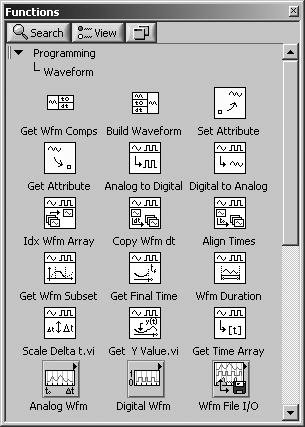
Waveform Functions

In the Functions palette, you'll find an entire subpalette beneath the Programming category dedicated to the waveform manipulation, aptly named Waveform (see Figure 8.70).

Figure 8.70. The Waveform palette

The Get Waveform Components and Build Waveform functions are used to get and set components of the analog waveform, digital waveform, and digital data.

Returns the waveform components you specify. You specify components by right-clicking and selecting Add Element and creating an indicator. This function is expandable.

Figure 8.71. Get Waveform Components

Builds a waveform or modifies an existing waveform. If you do not wire an input to waveform, Build Waveform creates a new waveform based on the components you enter. If you do wire an input in waveform, the waveform is modified based on the components you specify. This function is expandable.

Figure 8.72. Build Waveform

These two functions are polymorphic and can operate on analog waveforms, digital waveforms, and digital data. The waveform symbol on these functions will change depending on the data type wired to the waveform input. The analog waveform symbol looks like a small sine wave and the digital waveform symbol looks like a small square wave. You will see these same symbols on waveform functions, VI icons, and elsewhere. So keep a sharp eye out for themthey will help you identify which waveform data type you are working with.

The Waveform palette also has subpalettes with many useful functions and operations you can perform on waveforms.

The VIs in the Analog Waveform palette are used to perform arithmetic and comparison functions on waveforms, such as adding, subtracting, multiplying, finding the max and min points, concatenating, and so on (see Figure 8.73). Note that in most waveform operations that involve two or more waveforms, the waveforms involved must all have the same dt values.

Figure 8.73. Analog Waveform palette

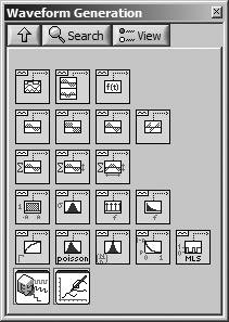
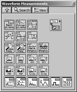
Analog Waveform Symbol

The Analog Waveform>>Waveform Generation palette allows you to generate different types of single and multitone signals, function generator signals, and noise signals (see Figure 8.74). For example, you can generate a sine wave, specifying the amplitude, frequency, and so on.

Figure 8.74. Waveform Generation palette

The Analog Waveform>>Waveform Measurements palette allows you to perform common time and frequency domain measurements such as DC, RMS, Tone Frequency/Amplitude/Phase, Harmonic Distortion, SINAD, and Averaged FFT measurements (see Figure 8.75).

Figure 8.75. Waveform Measurements palette

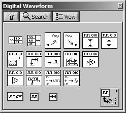
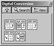
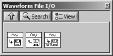
Digital Waveform Symbol

The Digital Waveform palette allows you to perform operations on digital waveforms and digital data, such as searching for digital patterns, compressing and uncompressing digital signals, and so on (see Figure 8.76).

Figure 8.76. Digital Waveform palette

The Digital Waveform>>Digital Conversion palette allows you to convert to and from digital data (see Figure 8.77).

Figure 8.77. Digital Conversion palette

The functions in Waveform File I/O allow you to write waveform data to and read waveform data from files (see Figure 8.78).

Figure 8.78. Waveform File I/O palette

One last thing you should know about waveformswhen you need to plot an analog waveform, you can wire it directly to a waveform chart or a waveform graph. The terminal automatically adapts to accept a waveform data type and will reflect the timing information on the X axis. Digital waveforms have their own digital waveform graph, which we will discuss later.

Let's look at a simple example of how to use and plot a waveform in the next activity.

Activity 8-6: Generate and Plot a Waveform

In this activity, you will generate a sine waveform, set its initial time stamp to the current time, and plot it on a chart.

1.	Open a new front panel.
2.	On the front panel, place a dial (from the Numeric palette), a chart, and a waveform indicator. Label the dial frequency, change its maximum value, and set it to 1 digit of precision (from the Format and Precision pop-up menu option), so that it looks like Figure 8.79. Figure 8.79. Front panel of the VI you will create during this activity

3.	Build a block diagram that will generate a sine waveform and plot it. The waveform generation functions do not provide a value for the t0 component of the waveform (they return the default time stamp value of 00:00:00.000 PM, MM/DD/YYYY, which, when converted to a DBL floating point in absolute time display mode, is midnight GMT 1/1/1904 (7:00:00 PM EST 12/31/1903), so use the Build Waveform to set the t0 to the current time. Here are the functions you will use the following: Sine Waveform.vi generates a waveform containing a sine wave with a null time stamp (00:00:00.000 PM, MM/DD/YYYY, or midnight GMT 1/1/1904 if represented as a DBL floating point in absolute time display mode). See Figure 8.80. Figure 8.80. Sine Waveform.vi The Get Date/Time in Seconds returns the current system date and time, as a time stamp data type (see Figure 8.81). Figure 8.81. Get Date/Time in Seconds

This function allows you to modify components of the waveform; in this activity, just t0 (see Figure 8.82).

Figure 8.82. Build waveform

Your block diagram should look like Figure 8.83.

Figure 8.83. Block diagram of the VI you will create during this activity

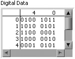
4.	Run and test your VI at different frequencies. You may want to pop up on the chart and select X Scale>>Autoscale X and Y Scale>>Autoscale Y. In addition, clearing the chart (by selecting Data Operations>>Clear Chart from its pop-up menu) between runs will make it more intelligible.
5.	Save your VI as `Waveform Exercise.vi.`

We'll take another look at waveforms again in Chapter 11, where the analog waveform data type is used in some of the analog input data acquisition functions.

Digital Data

Digital waveforms have a special data type for the Y component: a table of binary states (binary values can be either 0 or 1)the columns in the table are the digital lines and the rows are the successive values.

You can create a Digital Data control on the front panel from the I/O palette (Figure 8.84). The corresponding block diagram representation is a green terminal (Figure 8.85).

Figure 8.84. Digital data control

Figure 8.85. Digital data terminal

Digital Data Symbol

Note the digital data symbol on the digital data terminal, which looks like binary data (0101). This symbol is also found on functions and VIs that operate on digital data.

To easily convert to and from digital data, use the VIs located on the Programming>>Waveform>>Digital Waveform>>Digital Conversion palette (shown in Figure 8.86). These VIs allow you to convert digital data to and from Boolean arrays and Integer arrays, as well as import digital data from a spreadsheet string.

Figure 8.86. Digital Conversion palette

You can also operate on digital data using the Get Waveform Components and Build Waveform functions (which are also used to operate on waveforms), but this is not recommended.

Digital Waveform Graphs

For displaying digital waveform data, use the digital waveform graph (from the Modern>>Graph), as shown in Figure 8.87. If you've worked with digital logic before, the digital waveform graph isn't hard to use; otherwise, don't even worry about learning it! You can find some good examples on using digital waveform graphs in LabVIEW's built-in examples (examples\general\graphs\DWDT Graphs.llb).

Figure 8.87. Digital waveform graph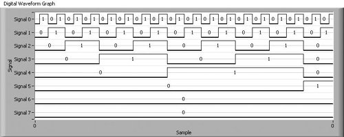

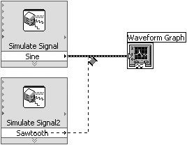
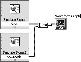
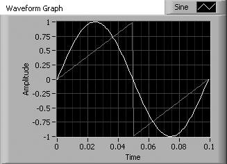
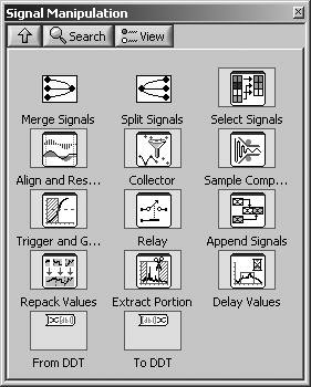
Dynamic Data

Nearly all of the Express VIs for acquiring, analyzing, manipulating, and generating signals use a special data type, called the dynamic data type, for passing signal data. Dynamic data is simply one or more channels of waveform datain fact, you can think of dynamic data as simply an array of analog waveforms, wrapped in a very smart wire. However, dynamic data is very smart, in that it makes it very easy for you to perform operations like merging signals into a single wire. For example, you can wire dynamic data directly to other dynamic data, and LabVIEW will automatically insert a Merge Signals function to combine the two signals into a single wire, as shown in Figure 8.88 and Figure 8.89.

Figure 8.88. Wiring dynamic data to an existing dynamic data wire (before)

Figure 8.89. Wiring dynamic data to an existing dynamic data wire (after)

If we look at a graph of our merged signal, shown in Figure 8.90, you can see that the resulting merged signal contains both a Sine signal and a Sawtooth signal.

Figure 8.90. Waveform graph displaying two dynamic data plots

The basic functions for manipulating dynamic data are found on the Express>>Signal Manipulation palette, shown in Figure 8.91. Here you will find functions for merging, splitting, and selecting signals, as well as the To DDT and From DDT functions, which are used to convert to and from traditional LabVIEW data types like waveforms, arrays, and scalars.