The Basic Transformations

When you are thinking about transformations, you can think about them in two different ways. On one hand you can think about applying a transformation to a set of objects to actually change the geometry of those objects. Drawing the object with the modified geometry redraws the object in a new location. This concept is illustrated in Figure 5.1.

Figure 5.1. Transforming Objects

In Figure 5.1, the staff is defined using some simple geometrical shapes. The shapes in the left side of the window represent the untransformed version of this particular geometry. The transformation chosen rotates the objects counterclockwise then moves them upward and to the right. The right side of Figure 5.1 shows the shapes after applying this transformation to them. In this case, the coordinate system has remained fixed, and the graphics have changed. We used a transformation to change the points that define the shape.

In addition to transforming geometry, you also can transform the coordinate system. This idea is a bit more difficult to understand. In the physical world, everyone is used to manipulating objects, we're not as accustomed to changing coordinate systems.

When transforming a coordinate system, you must have another coordinate system to compare it to. The transformation provides a relative mapping from one coordinate system to the other. When you draw in the transformed coordinate system, the transformation maps the graphic back to the first coordinate system. The appearance of that graphic in the fixed coordinate system is affected by the transformation. Figure 5.2 illustrates the results of using a transform to define a new coordinate system.

Figure 5.2. Transforming Coordinates

In the left half of Figure 5.2, is a graphic whose geometry defines shapes that are close to the origin. A transformation is then used to define a new, relative coordinate system. The transform rotates the coordinate axes 30 degrees clockwise and then shifts the origin upward and to the right. The transformations are relative to the original coordinate frame. Now you can redraw the exact same graphic in this new coordinate system.

The geometry that defines the shape of the graphic does not change. The points that define the shape still draw close to the origin and at the same orientation relative to the coordinate axes. However, when viewed from the perspective of our fixed coordinate system (represented in the gray arrows in Figure 5.2), the graphic appears to have changed both location and orientation.

Quartz 2D allows you to use transformations in both of these capacities. You can construct geometric objects and then modify the points that define those shapes by applying transformations to them. Alternatively, you can create transformations that help you define alternate coordinate systems and apply those transforms (e.g., to user space) to set up convenient drawing environments.

An important, albeit difficult, thing to realize about these two perspectives on transformations is that they are just two ways of looking at the same thing. Your application can create transformations that it applies to the coordinate system to get the exact same end results it might get from transforming the geometry that makes up the graphic. As a programmer you have the flexibility to choose the particular perspective on a transformation that simplifies the drawing task at hand. By the same token if you find yourself struggling to create a transformation to achieve a particular effect, you might try looking at the transformation from the other perspective and see if the new eyes help.

Affine Transform

Up to this point we have been talking about general transformations. Quartz 2D does not support arbitrary 2D transformations. Instead, the library supports a very particular sub-set of those transformations. The set of transformations Quartz 2D supports are known as affine transforms.

Affine transformations have a very rigorous and very specific meaning to mathematicians. We won't bore you with that definition here, as understanding the definition would probably not help you understand how to use transformations in Quartz 2D.

There are some interesting properties of affine transformations that are worth mentioning. First of all, if you have a set of points that all lie on the same line (they are colinear) and you apply an affine transformation to those points, you will find that the transformed points are also colinear. The affine transformation will also preserve the relative distances between the points. If you have any lines in your geometry that are parallel to one another, the lines will still be parallel after you transform them.

The fact that affine transformations preserve the parallel relationships between lines makes them unsuitable for general perspective transformations. In other words, the transformations in Quartz 2D cannot be used for the perspective projections commonly associated with rendering 3D graphics. This also means that you cannot use Quartz 2D graphics to achieve effects that involve destroying parallelism. You cannot, for example, use an affine transformation to taper a rectangle at one end.

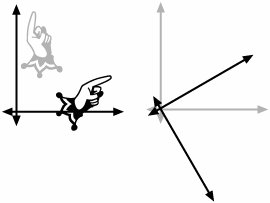
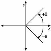
Affine transforms have another useful property. You can combine simple affine transformations to create more complex ones. If you transform a set of points with the combined transformation, the net effect will be the same as if you had transformed those points with one of the component transformations first and then passed the results through the second component transformation. The result of combining any two affine transformations is also an affine transformation.

Quartz 2D exploits this fact by providing simple transformations whose effects you can visualize easily. The library also gives your application the tools it needs to combine the simple transformations together. The three basic transformation types that Quartz 2D supports are Translations, Rotations, and Scalings. We will demonstrate each transformation shortly and then show you how to use the Quartz 2D APIs to combine them.

Translations

Translation is a very fancy term for moving a thing from one location to another. When you translate your geometry, you move the points in the geometry to somewhere else in the coordinate space. From the perspective of mapping the coordinate system, a translation offsets the origin of the coordinate system to a new location. Figure 5.3 illustrates the effects of applying translations.

Figure 5.3. Translations Viewed in Two Ways

In the left side of Figure 5.3 a translation has been applied to the geometry of a star-shaped graphic. The grey version of the star is the geometry before the translation is applied, and the black star is the geometry after translating it. In the left side of the figure, we have translated a coordinate system. The origin of the transformed coordinate system is offset from the origin of the reference coordinate system by a bit.

To specify a translation, your code specifies the offset you want to apply in the x and y coordinate directions.

Rotations

Rotations allow you to change the orientation of a graphic or to change the relative orientations of two coordinate systems. The fundamental rotational affine transform is a rotation around the origin. If you want to rotate around a different point in space, you have to combine the rotation with a transformation. The idea is revisited later in the discussion about how to combine the primitive transformations. Figure 5.4 demonstrates the effects of applying a rotation.

Figure 5.4. Rotations Illustrated

In the figure a counter-clockwise rotation of 60 degrees has been applied to both a graphic, on the left, and a coordinate system, on the right. The gray illustration shows the original position of the graphic and the coordinate axes. The black graphics are the locations after rotation. The pivot point of each rotation is the origin. Because the hand graphic in the left side of the figure is not centered on the origin, the hand not only turns, but it also moves laterally through space.

To specify a rotation, you simply provide the computer with the angle through which you would like to rotate the object or axes. In Quartz 2D angles are measured according to the diagram in Figure 5.5.

Figure 5.5. Measuring Rotations

Figure 5.5 shows that positive angles are measured in the direction from the positive x axis to the positive y axis. Negative angles, of course go the other way. You should avoid thinking that positive angles turn things counter clockwise and negative angles rotate them clockwise. Quartz can orient the coordinate systems arbitrarily. If an application reverses the direction of either axis (using a scaling transform with a negative scaling factor, see below), you will also reverse the relationship between the angle's sign and the clockwise/counterclockwise directions. Carbon programmers working with the coordinate system passed to them by HIView are working with a coordinate system where the y axis has been reversed in this fashion.

Degrees versus Radians

When supplying the angles used to specify rotations, you need to pay attention to the different angle measurement units. Core Graphics routines accept angles in radians, while the Cocoa routines typically accept angles in degrees.

As a quick refresher, a full circle is 360 degrees (360°) which is equivalent to 2p radians. If you want to convert between degrees and radians, you can use the formula

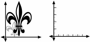
Scaling

Scaling a graphic makes it larger or smaller. Scaling one coordinate system relative to another changes the relative distances covered by one unit along each of the axes.

Like rotation, the computer applies scales relative to the origin. If you scale objects that are not centered at the origin, the objects will move as well. This happens when the computer scales the space between the object and the origin in addition to the objects themselves. The effects of a scaling transformation are illustrated in Figure 5.6.

Figure 5.6. Scaling Objects and Coordinates

In Figure 5.6 the axes have been scaled independently of one another. When you specify a scale in Quartz 2D, you provide the scaling factor for each of the axes separately. In the figure, we used a scale of 2.25x (or 225%)2.25x (or 225%) on the y axis and a scaling factor of 1.5x (150%)1.5x (150%) to the x axis. On the left side we see the effects of scaling a graphic by our scaling factor. As in the previous figures, the gray object represents the object prior to applying the transformation, and the black object shows the transformed object.

The right half of Figure 5.6 shows the effect of scaling a coordinate system and deserves some explanation. Scaling a coordinate system changes the distance covered by each unit of the coordinate system. To illustrate this, the right side of Figure 5.6 includes marks at one unit intervals along each of the axes. The gray marks show the unit marks for the unscaled coordinate system. The black marks, of course, show the unit marks of the coordinate system after scaling. Note that along the y axis, the first scaled tick mark draws after two and 1/4 marks on the unscaled axis. Similarly, the first x tick mark on the scaled interface is found after one and a half tick marks on the unscaled axis.

Scaling an axis by 1.0 has no effect on the axis whatsoever. Scaling by a value larger than 1 increases the distance between coordinate units. This makes objects drawn in that coordinate system larger. Scaling by a value greater than 0 but less than 1 shortens the distance between coordinate units. This shrinks objects that are drawn to the fixed coordinate system. Scaling by a scale factor of 0 is meaningless, and the behavior of the system (as well as the math) is not well defined.

Interesting things happen when you scale an axis by a negative value. The scale not only changes the relative lengths of units, but it also reverses the direction of the corresponding axis. This can be very convenient if you want to convert the Quartz 2D coordinate system so that it matches the coordinate system of other graphics libraries such as QuickDraw or GDI. To accomplish this transformation, however, you have to combine this scaling factor with a translation. An example of this kind of transformation appears later in the chapter.

Inverse Transformations

Before discussing combining transformations, the inverse of transformations should be considerd. If you think of transformations as an operation that has an particular effect on a graphic, then the inverse transformation would be a transformation that exactly undoes that effect.

The inverse transformation of a translation by 100 pixels on the x axis and 50 pixels on the y axis would be a translation of -100 pixels on the x axis and -50 pixels on the y axis. If you moved a graphic using the first set of offsets and then moved it again by the second set, you would be putting the graphic back in its original location.

The inverse of rotation by an angle is rotation by the same angle in the opposite direction. This is equivalent to using an angle of the same magnitude, but opposite sign. If you rotate a graphic by 30 degrees, the inverse transformation is a rotation by -30 degrees.

The inverse of scaling the coordinate system by the factor S is scaling the coordinate system by the factor . If you scale a coordinate system by 2, the inverse transformation will be a scale by ½.

You can use these facts to create your own inverse affine transformations. Quartz 2D also includes a routines to invert affine transformations.

Concatenating Transformations

Combining transformations is little more than applying one transformation after another to either a graphic or coordinate system. If you were to take your geometry and pass it through a series of transformations individually, you would not only incur the computational expense of each transformation, but you would be more likely to find that small mathematical errors would creep into the calculations. To avoid this, Quartz 2D uses matrix multiplication to concatenate a long chain of transformations into a single matrix.

As an example of this process consider the task of rotating a graphic about its center when the graphic is not originally located at the origin. This process is illustrated in Figure 5.7.

Figure 5.7. Rotating a Graphic About its Center

In this case we're going to accomplish our rotation by combining three different transformation steps. Figure 5.7(a) shows the graphic, an umbrella, in its initial position. The goal is to rotate this graphic about its center by 30 degrees. Recall, however, that the rotation primitive only rotates objects around the origin. What is needed is to center the umbrella on the origin by using a translation (Figure 5.7(b)), rotate it (Figure 5.7(c)), and then move it back to it's original location with another translation (Figure 5.7(d)).

If the umbrella figure has its center at (100, 100), then the following code snippet represents the steps needed to transform the umbrella:

CGAffineTransform affineTransform = CGAffineTransformIdentity; affineTransform = CGAffineTransformConcat(                    affineTransform,                    CGAffineTransformMakeTranslation(-100, -100)); affineTransform = CGAffineTransformConcat(                    affineTransform,                    CGAffineTransformMakeRotation(pi / 6)); affineTransform = CGAffineTransformConcat(                    affineTransform,                    CGAffineTransformMakeTranslation(100, 100)); CGPathRef transformedPath = CopyPathWithTransformation(                    umbrellaPath, affineTransform); 

This code snippet begins by creating a CGAffineTransform structure and initializes it with the identity transform. The identity transform is just a starting place. If you take a graphic and transform it by the identity transform, you simply get back the original graphic.

From there it concatenates together the three transformations we want to apply to our umbrella. The first is the translation by (-100, -100). This moves the center of the umbrella to the origin. Next is the rotation by 30 degrees that turns the umbrella about the origin. Finally the object is put back where it was found by translating by (100, 100) a copy of the transformed umbrella is then created using a self-devised utility routine called CopyPathWithTransformation.

This is a fairly simple example of combining transforms. Your application can create any affine transformation that Quartz 2D supports by combining the three basic transformations in this fashion. Learning to do this effectively takes a little imagination and a lot of practice. When you grasp the concepts, however, it becomes much easier to use transformations to your advantage.

If you concatenate the inverse of a particular transform with the transform itself, you should get back the identity transform. In a computer with infinite floating point precision, if you were to apply a particular transform to the graphics context, you would be able to undo that transformation by applying the inverse transformation to the context as well.

Unfortunately, computers represent floating point numbers with limited precision. As a result, combining a matrix with its inverse does not always result in an identity matrix. Small errors can creep into the mathematics. These errors can affect the graphics you draw with the resulting transformations.

Instead of calculating inverse transformations, you should use the CGContextSaveGState and CGContextRestoreGState routines to save and restore the graphics state (which will also save and restore the CTM). This will ensure that the old transformation matrix is retrieved exactly as it was.

The Order Matters

When you are concatenating transformations together, you have to combine them in the proper order. This can be a bit tricky because the Quartz 2D API includes a couple of different sets of routines for combining transformations, and you may have to modify the order of your routine calls depending on which set of routines you are using.

The order that you use transformations is important because scalings and rotations happen relative to the origin. To illustrate this difference, let us look at what happens if we reverse the first two steps of our umbrella's journey. Figure 5.8 shows the umbrella if we first rotate it and then translate it.

Figure 5.8. Applying Transforms in the Wrong Order

To make Figure 5.8, we started with the figure in 5.7(a) and then applied the first two transformations in the opposite order. That means that Figure 5.8(a) shows the effect of rotating the umbrella by 30 degrees. Figure 5.8(b) shows the graphic if we subsequently offset the umbrella by (-100, -100). Compare these two pictures with the graphics of Figure 5.7(b) and 5.7(c). Because you cannot reverse the order of transformations without affecting the final image, Figure 5.8(b) is very different from 5.7(c).

The reason for the discrepancy is the fact that the basic rotation transform uses the origin as its pivot point. That means that when the umbrella is not centered on the origin, any rotation also moves the umbrella laterally across the canvas. When you combine that lateral motion with the transform, you find that the umbrella is in a different position. Scaling transformations would have a similar effect. If you apply a scaling transformation, you scale not only the object itself, but the space between the object and the origin. That means that scaling the object also moves it.

This leads to the observation that you have to be very careful about ordering your transformations when you try to combine scaling and rotations with translations. The order in which you apply your transformations can also be important depending on which Quartz APIs you are using to combine the basic transforms. In our previous code snippet, we used the Quartz 2D routine CGAffineTransformConcat. This routine works well for combining two existing transformations but requires us to create a transformation at each step. In that example CGAffineTransformConcat was chosen because it allowed demonstration of creating a transform from basic transforms by combining the individual steps in a logical order. The same transformation, however, can be accomplished with a bit less code. Consider the calling sequence

CGAffineTransform affineTransform = CGAffineTransformIdentity; affineTransform = CGAffineTransformTranslate(affineTransform, 100, 100); affineTransform = CGAffineTransformRotate(                           affineTransform, pi / 6); affineTransform = CGAffineTransformTranslate(                           affineTransform, -100, -100); CGPathRef transformedPath = CopyPathWithTransformation(                                   umbrellaPath, affineTransform); 

This calling sequence accomplishes the exact same transformation that the previous code snippet accomplished and does not require the CGAffineTransformMakeXXX routines. What you should notice, however, is the fact that this code reverses the order in which the transformations are combined. This is a consequence of the way mathematics combines the transformation. When looking at this code, you might choose to think that the last transformation applied to the affineTransform structure is the first transformation applied to the object.