Using Filters

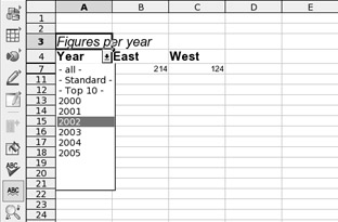
The Filter function in Calc lets you selectively hide rows of data. The spreadsheet user then selects which of the rows of data to view from a drop-down list that appears in the cell at the top of the rows, as shown in the example in Figure 25-5.

Figure 25-5. Filters allow you to selectively hide or show rows of data in a spreadsheet.

Note 

A Calc filter is a little like an Excel pivot chart, especially when it's combined with an automatically generated chart.

Using filters in this way can be useful when you're dealing with a very large table of data. It helps isolate figures so you can compare them side by side in an easy-to-follow format. For example, you could filter a table of sales figures by year.

To use the Filter function, start by highlighting the data you wish to see in the drop-down list. Make sure the column header for the data is included, too. If you're using the Filter feature on a table of data, this selection can be any column within the table, although it obviously makes sense to use a column that is pertinent to the filtering that will take place. After you've selected the data to filter, select Tools ® Filter ® Autofilter. You should find that, in place of the column header, a drop-down list appears. When a user selects a various entry in the list, Calc will display only the corresponding row of the spreadsheet beneath.

To remove a filter, select Tools ® Filter ® Hide Autofilter.