 [Page 194 ( continued )] [Page 194 ( continued )] Some of the most interesting and useful applications of integer programming involve 01 variables. In these applications the variables allow for the selection of an item (or activity) where a value of one indicates that the item is selected and a value of zero indicates that it is not. For example, a decision variable might represent the purchase of a building; if the value of the variable is one, the building is purchased. If the value is zero, the building is not purchased. We will demonstrate three of the most popular applications of 01 integer programminga capital budgeting problem, a fixed charge and facility location problem, and a set covering problem. A Capital Budgeting Example The University Bookstore at Tech is considering several expansion projects, including developing a store Web site for online retail and catalog purchases, buying an off-campus warehouse and its subsequent expansion, developing a clothing and gift department specializing in university logo apparel, opening a computer department carrying both hardware and software products, and creating a banking pavilion of three automated teller machines outside the store. Some of the projects will be developed over a 2-year period and some over a 3-year period, as funds permit. The net present value costs per year and the projected net present value of returns for a 5-year period for each of the projects are shown in the following table:
[Page 195] | | | Project Costs/Year ($1,000s) | | Project | NPV Return ($1,000s) | 1 | 2 | 3 | | 1. Web site | $120 | $55 | $40 | $25 | | 2. Warehouse | 85 | 45 | 35 | 20 | | 3. Clothing department | 105 | 60 | 25 | | | 4. Computer department | 140 | 50 | 35 | 30 | | 5. ATMs | 70 | 30 | 30 | | | Available funds per year | | $150 | $110 | $60 |
Management Science Application: Optimal Assignment of Gymnasts to Events (This item is displayed on page 194 in the print version) An integer programming model was developed to assign members of a women's gymnastics team to the four events conducted at a typical NCAA meetvault, uneven bars, balance beam, and floor exercises. Each team can enter up to six gymnasts in each event, and the top five scores among these entrants contribute to the team score. At least four of the entrants must participate in all four events. These conditions formed the model constraints; the objective was to maximize the team's overall expected score. The model was tested at Utah State University and allowed officials to analyze the effects of changing conditions, such as improved performance or injuries, on the team score; to indicate to a team member why she was not selected for a particular event; and to eliminate the time the coach spent manually evaluating different team combinations.  Source: P. Ellis and R. Corn, "Using Bivalent Integer Programming to Select Teams for Intercollegiate Women's Gymnastics Competition," Interfaces 14, no. 3 (MayJune 1984): 4146. |
In addition, the store does not have enough space available to create both a computer department and a clothing department. The bookstore director wants to know which projects to select to maximize returns. This problem requires a 01 integer programming model formulation where x 1 = selection of Web site project x 2 = selection of warehouse project x 3 = selection of clothing department project x 4 = selection of computer department project x 5 = selection of ATM project x i = 1 if project i is selected; 0 if project i is not selected 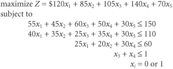 Exhibit 5.16 shows this capital budgeting example set up in Excel spreadsheet format. The decision variables for the projects are in cells C7:C11 , and the objective function ( Z ) is in cell D17. The objective function is shown on the formula bar at the top of the spreadsheet. The model constraints are included in cells E12:G12 . For example, cell E12 contains the budget constraint for year 1, = SUMPRODUCT (C7:C11, E7:E11) , and the available budget is in cell E14. Thus, this budget constraint will be written in Solver as E12  E14 . The mutually exclusive constraint, x 3 + x 4 1, is included in cell E15 as = C9+C10 . E14 . The mutually exclusive constraint, x 3 + x 4 1, is included in cell E15 as = C9+C10 . Exhibit 5.16. (This item is displayed on page 196 in the print version) 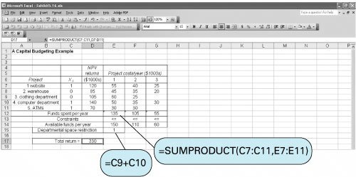
Exhibit 5.17 shows the Solver screen for the capital budgeting example. The 01 variable restriction has been established by the constraints C7:C11 1 and C7:C11 = integer . The mutually exclusive constraint is shown as E15 1 .
[Page 196] Exhibit 5.17. 
The model solution is x 1 = 1 (Web site) x 4 = 1 (computer department) x 5 = 1 (ATMs) Z = $330,000 A Fixed Charge and Facility Location Example Frijo-Lane Food Products own farms in the Southwest and Midwest, where it grows and harvests potatoes. It then ships these potatoes to three processing plants in Atlanta, Baton Rouge, and Chicago, where different varieties of potato products, including chips, are produced. Recently, the company has experienced a growth in its product demand, so it wants to buy one or more new farms to produce more potato products.
[Page 197] The company is considering six new farms with the following annual fixed costs and projected harvest: | Farm | Fixed Annual Costs ($1,000s) | Projected Annual Harvest (thousands of tons) | | 1 | $405 | 11.2 | | 2 | 390 | 10.5 | | 3 | 450 | 12.8 | | 4 | 368 | 9.3 | | 5 | 520 | 10.8 | | 6 | 465 | 9.6 |
The company currently has the following additional available production capacity (tons) at its three plants, which it wants to utilize: | Plant | Available Capacity (thousands of tons) | | A | 12 | | B | 10 | | C | 14 |
The shipping costs ($) per ton from the farms being considered for purchase to the plants are as follows : | | Plant (shipping costs, $/ton) | | Farm | A | B | C | | 1 | 18 | 15 | 12 | | 2 | 13 | 10 | 17 | | 3 | 16 | 14 | 18 | | 4 | 19 | 15 | 16 | | 5 | 17 | 19 | 12 | | 6 | 14 | 16 | 12 |
The company wants to know which of the six farms it should purchase to meet available production capacity at the minimum total cost, including annual fixed costs and shipping costs. This problem is formulated as a 01 integer programming model because the selection of the farms requires 01 decision variables: y i = 0 if farm i is not selected, and 1 if farm i is selected, where i = 1, 2, 3, 4, 5, 6 The variables for the amounts shipped from each prospective farm to each plant are non- integer, defined as follows: x ij = potatoes (tons, 1,000s) shipped from farm i to plant j , where i = 1, 2, 3, 4, 5, 6 and j = A, B, C
[Page 198] The objective function ( Z ) combines shipping costs and the annual fixed costs, where Z = $1,000s: 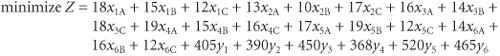 The constraints for production capacity require that potatoes be shipped (i.e., x ij variables have positive values) only from a farm if it is selected; for example, for farm 1, x 1A + x 1B + x 1C 11.2 y 1 In this constraint, if y 1 = 1, then the 11.2 thousand tons of potatoes are available at farm 1 for shipment to one or more of the plants. Similar constraints are developed for each of the five other farms. Constraints are also necessary for the production capacity to be filled at each plant. The complete model is formulated as  subject to 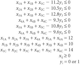 Exhibit 5.18 shows this example model set up in Excel spreadsheet format. The decision variables for the shipments between farms and plants, x ij , are in cells C5:E10 . The 01 decision variables for farm selection, y i , are in cells C17:C22 . The objective function ( Z ) is embedded in cell C24 and is shown on the formula bar at the top of the spreadsheet. The model constraints for potato availability at the farms are embedded in cells H5:H10 . For example, the total amount shipped from farm 1, x 1A + x 1B + x 1C , is in cell G5 as = C5+D5+E5 . The constraint formulation is in cell H5 as = G5C17 * F5 . The constraints for potatoes shipped from the plants are in cells C12:E12 . For example, the constraint formula in C12 is = SUM (C5:C10) . Exhibit 5.18. (This item is displayed on page 199 in the print version) 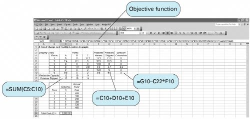
Exhibit 5.19 shows the Solver screen for this example. The 01 variable restriction for the y i variables is established by the constraints C17:C22 1 and C17:C22=integer . The farm harvest (potato availability) constraints are shown as H5:H10 , and the plant production capacity constraints are shown as C12:E12=C11:E11 . Exhibit 5.19. (This item is displayed on page 199 in the print version) 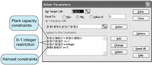
The model solution is 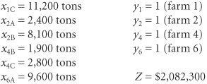
[Page 199] A Set Covering Example American Parcel Service (APS) has determined that it needs to add several new package distribution hubs to service cities east of the Mississippi River. The company wants to construct the minimum set of new hubs in the following 12 cities so that there is a hub within 300 miles of each city (i.e., every city is covered by a hub):
[Page 200] | City | Cities Within 300 Miles | | 1. Atlanta | Atlanta, Charlotte, Nashville | | 2. Boston | Boston, New York | | 3. Charlotte | Atlanta, Charlotte, Richmond | | 4. Cincinnati | Cincinnati, Detroit, Indianapolis, Nashville, Pittsburgh | | 5. Detroit | Cincinnati, Detroit, Indianapolis, Milwaukee, Pittsburgh | | 6. Indianapolis | Cincinnati, Detroit, Indianapolis, Milwaukee, Nashville, St. Louis | | 7. Milwaukee | Detroit, Indianapolis, Milwaukee | | 8. Nashville | Atlanta, Cincinnati, Indianapolis, Nashville, St. Louis | | 9. New York | Boston, New York, Richmond | | 10. Pittsburgh | Cincinnati, Detroit, Pittsburgh, Richmond | | 11. Richmond | Charlotte, New York, Pittsburgh, Richmond | | 12. St. Louis | Indianapolis, Nashville, St. Louis |
This problem requires a 01 integer programming model in which the decision variables are the available cities: x i = city i , i = 1 to 12 where x i = 0 if city i is not selected as a hub and x i = 1 if city i is selected The objective function ( Z ) is to minimize the number of hubs: minimize Z = x 1 + x 2 + x 3 + x 4 + x 5 + x 6 + x 7 + x 8 + x 9 + x 10 + x 11 + x 12 Management Science Application: Managing Prototype Vehicle Test Fleets at Ford Ford Motor Company, with 350,000 employees in 111 manufacturing plants in 38 countries , is the second-largest manufacturer of cars and trucks in the world. The product design process at Ford is a time-consuming and extremely expensive process, and designs must be painstakingly verified . For the verification of some designs, a prototype vehicle must be constructed , at a cost routinely exceeding $250,000. Prototypes are costly because most of the parts and assembly processes are unique, and the tools that would eventually be used in mass production do not exist yet. Complex vehicle development programs often require more than 100, and sometimes more than 200, vehicle prototypes. Because the cost of developing prototype vehicles depends solely on the number built, the goal is to build as few prototypes as possible to perform the required testing. A group of students and faculty associated with the 3-year engineering master's program at Wayne State University developed the prototype optimization model (POM) to reduce the number of prototype vehicles Ford needed to verify its product designs. Initially a group of students in this program (who were also engineering managers at Ford) noticed a conceptual similarity between a class set covering example and the problem of developing a prototype fleet to cover a set of required tests. These students undertook the prototype-planning problem as their team project required in the master's program. This group developed a hypothetical data set and model, and students in the next graduating class picked up where they left off to eventually develop POM. The model's objective was to determine the minimum number of prototype vehicles required to complete every verification test by a specific deadline. This requires that prototype vehicles be shared among design groups, thereby increasing the usage of vehicles and reducing the time they sit idle, waiting for testing. In the first step in POM, a set covering problem is formulated to determine the minimum number of unique vehicle configurations needed to cover all the tests. A list of every realistic vehicle configuration, called the building combination matrix (BCM), is developed. An actual design could initially include more than 1,000 possible vehicle configurations. POM was first used for the European Transit vehicle program. It began with 38,880 possible combinations, and the model identified a set of 27 unique vehicle configurations required to cover all the tests, offering a cost savings of $12 million. Ford has since used POM to budget, plan, and manage more than 10 complex vehicle design programs, including those for Taurus, Windstar, Explorer, and Ranger. The overall costs for prototype vehicles were reduced by more than $250 million from 1995 to 2000.  Source: K. Chelst, J. Sidelko, A. Przebienda, J. Lockledge, and D. Mihailidis, "Rightsizing and Management of Prototype Vehicle Testing at Ford Motor Company," Interfaces 31, no. 1 (JanuaryFebruary 2001): 91107. |
[Page 201] The model constraints establish the set covering requirement (i.e., that each city be within 300 miles of a hub). For example, Atlanta covers itself, Charlotte, and Nashville: Atlanta: x 1 + x 3 + x 8  1 1 In this constraint, at least one of the variables must equal 1 in order for Atlanta to be assured of a hub within 300 miles. Similar constraints are developed for the other 11 cities. The complete 01 integer programming model is summarized as follows: 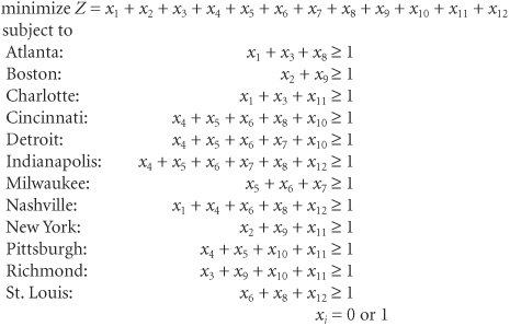 The Excel spreadsheet for this model is shown in Exhibit 5.20. The decision variables for the cities and hub sites are in cells B20:M20 , and the objective function ( Z ) is in cell B22. The formula for the objective function embedded in B22 is the sum of the cities selected as hubs, = SUM (B20:M20) . The model constraints are in cells N7:N18 . Notice that the values of 1 in cells B7, D7, and I7 indicate the cities covered by a possible hub at Atlanta. Exhibit 5.20. 
Exhibit 5.21 shows the Solver screen for this problem. The 01 variable restriction has been established by the constraints B20:M20 1 and B20:M20 = integer . Notice that the formulas in cells N7:N18 are set 1 (i.e., N7:N18 1 ) to complete the "set covering" constraints in the model.
[Page 202] Exhibit 5.21. 
Management Science Application: Planning Next-Day Air Shipments at UPS UPS is the leading package-delivery company in the world, each day delivering more than 13 million packages to 8 million customers in more than 200 countries. UPS Airlines, the ninth-largest commercial airline in the United States, with more than 345 aircraft, is the key component that enables the company to provide expedited (express) delivery service. The airline's next-day service delivers more than 1 million packages each night and annually generates over $5 billion in revenue. In the UPS air network, trucks transport originating packages to ground centers and from ground centers to more than 100 airports. Each plane carries its packages directly to one of 6 regional hubs (Columbia, SC, Dallas, TX, Hartford, CT, Ontario, CA, Philadelphia, PA, and Rockford, IL) or 1 all-points hub (in Louisville, KY), and it may stop at an airport along the way to pick up additional packages. Packages are sorted at the hubs and loaded onto aircraft for outbound delivery to a destination airport. At the destination airport, workers transfer the packages to trucks that move them to ground centers, where they are scanned, sorted, and loaded onto smaller trucks for delivery to their final destinations. Each type of aircraft has a maximum flying range, effective speed, landing restrictions at different locations, and cargo capacity. The maximum number of airports a plane can visit on a pickup or delivery route (not including a hub) is two. Planning a shipping network of this size with 7 hubs, more than 100 airports, more than 2,000 combinations of airport origin and destination pairs, and a huge volume of packages is a very large, complex problem. In 2000 the company implemented VOLCANO (Volume, Location, and Aircraft Network Optimizer) to determine aircraft routes, fleet assignments, and package routing to ensure overnight delivery at a minimum cost. VOLCANO is based on an integer programming set covering model formulation. This system saved the company more than $87 million between 2000 and 2002 by ensuring that it would use the most efficient routes with the fewest planes. UPS estimated that it would result in savings of more than $189 million over the next decade .  Source: A. P. Armacost, C. Barnharrt, K. A. Ware, and A. M. Wilson, "UPS Optimizes Its Air Network," Interfaces 34, no. 1 (JanuaryFebruary 2004): 1525. |
[Page 203] The model solution is 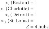 Notice that there is only one city covered by two hubs, Indianapolis (i.e., 2 in cell N12), which is overlapped by both Detroit and St. Louis. Also, there are multiple optimal solutions to this problem (i.e., different mixes of four hubs). |