Computer Solution of Integer Programming Problems with Excel and QM for Windows
| Integer programming problems can be solved using Excel spreadsheets and QM for Windows. In this section we demonstrate both of these computer solution approaches, using the examples for 01, total, and mixed integer programming problems developed in the previous sections. Solution of the 01 Model with ExcelRecall our recreational facilities example, formulated on page 182: where x 1 = construction of a swimming pool x 2 = construction of a tennis center x 3 = construction of an athletic field x 4 = construction of a gymnasium Z = total expected usage (people) per day Exhibit 5.2 shows this example model set up in Excel spreadsheet format. The decision variables for the facilities are in cells C12:C15 , and the objective function ( Z ) is embedded in cell C16. The objective function is shown on the formula bar at the top of the spreadsheet. The model constraints are contained in cells G7, G8, and G9. For example, cell G7 includes the cost constraint, = C7 * C12+D7 * C13+E7 * C14+F7 * C15 , and the available budget of $120,000 is contained in cell I7. Thus, the cost constraint will be written in Solver as G7 Exhibit 5.2.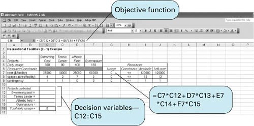 Exhibit 5.3 shows the Solver screen for our spreadsheet example. Notice that we have established the 01 condition of our variables by constraining the decision variable cells to be less than or equal to one (i.e., C12:C15 Exhibit 5.3.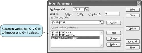
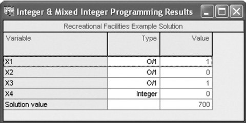
Next, we constrain the decision variables to be integer (i.e., C12:C15=integer ). The addition of this latter constraint is shown in Exhibit 5.4. These two constraints, along with the nonnegativity constraint ( C12:C15 Exhibit 5.4. Exhibit 5.5.(This item is displayed on page 189 in the print version)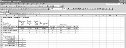 Solution of the 01 Model with QM for WindowsThe 01 integer programming problem is solved in the "Integer and Mixed Integer" module of QM for Windows. We will demonstrate this module by using our example for selecting recreational facilities that we just solved with Excel. Exhibit 5.6 shows the data input screen for our recreational facilities example problem. At the bottom of the screen, when you click on "Variable Type" for a variable, a menu will be displayed from which you can indicate if the variable is 01, integer, or real. In the case of this example, all the variables should be designated 01. The model is solved by clicking on the "Solve" button at the top of this screen, which results in the solution screen shown in Exhibit 5.7. Exhibit 5.6.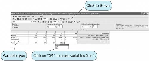 Exhibit 5.7.
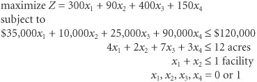
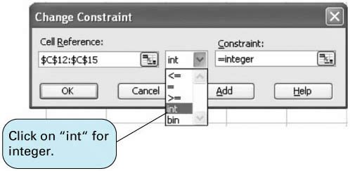
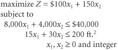
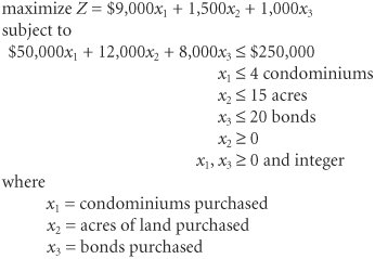
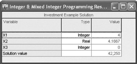
The solution shown in the QM for Windows output is x 1 = 1 swimming pool x 2 = 0 tennis center x 3 = 1 athletic field x 4 = 0 gymnasium Z = 700 people per day expected usage Solution of the Total Integer Model with ExcelWe will demonstrate the Excel solution of a total integer programming problem for the machine shop example we solved previously using the branch and bound method. Recall that this model was formulated as where x 1 = number of presses x 2 = number of lathes The machine shop example set up in spreadsheet format is shown in Exhibit 5.8. This is the same basic format as a linear programming model. The essential difference between solving a regular linear programming model and an integer programming model is that we must designate the cells representing the decision variables as being "integer." We accomplish this by adding a constraint within Solver that establishes B10:B11 as integers, as shown in Exhibit 5.10. The complete Solver, with all constraints, is shown in Exhibit 5.9. Clicking on the "Solve" button will generate the spreadsheet solution, as shown in Exhibit 5.11. Exhibit 5.8.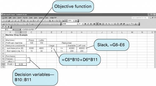 Exhibit 5.9.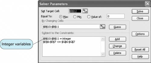 Exhibit 5.10. Exhibit 5.11.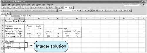 Solution of the Mixed Integer Model with ExcelThe solution of a mixed integer programming model with Excel will be demonstrated by using the example for investments formulated earlier in the chapter: where x 1 = condominiums purchased x 2 = acres of land purchased x 3 = bonds purchased The Excel spreadsheet solution is shown in Exhibit 5.12, and the Solver window is shown in Exhibit 5.13. The decision variables are contained in cells B8:B10 . The objective function formula is in cell B11 and is also displayed on the formula bar at the top of the spreadsheet. Notice that we did not include the constraint values for the availability of each type of investment (i.e., 4 condos, 15 acres of land, and 20 bonds) in the spreadsheet setup. Instead, it was easier just to enter these constraints directly into Solver, as shown in Exhibit 5.13. Notice in Solver that we have designated B8 and B10 as integers, but we have not designated B9 as an integer, reflecting the fact that x 1 and x 3 are integers, whereas x 2 is a real variable. Exhibit 5.12.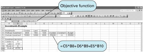 Exhibit 5.13.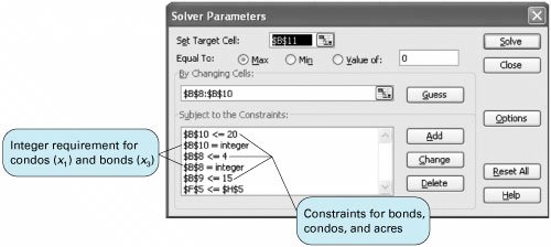 Solution of the Mixed Integer Model with QM for WindowsThe "Integer and Mixed Integer" module of QM for Windows is used to solve our investment example. When the problem data are input, we must designate the variable types for each decision variable. In this case, x 1 and x 3 are entered as integer variables, and x 2 is entered as a real variable. The QM for Windows input screen for our investment example is shown in Exhibit 5.14, and the solution screen is shown in Exhibit 5.15. Exhibit 5.14.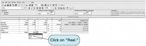 Exhibit 5.15. |


EAN: 2147483647
Pages: 358