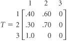
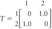
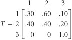
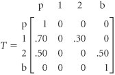
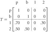
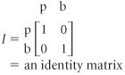
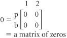
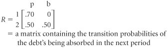
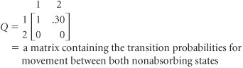
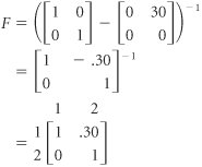
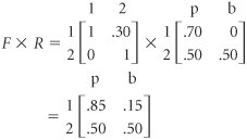
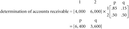
Special Types of Transition Matrices | Introduction to Management Science (10th Edition)

[Page F-13 ( continued )]

In some cases the transition matrix derived from a Markov problem is not in the same form as those in the examples shown in this chapter. Some matrices have certain characteristics that alter the normal methods of Markov analysis. Although a detailed analysis of these special cases is beyond the scope of this chapter, we will give examples of them so that they can be easily recognized.

In the transition matrix

state 3 is a transient state . Once state 3 is achieved, the system will never return to that state. Both states 1 and 2 contain a 0.0 probability of going to state 3. The system will move out of state 3 to state 1 (with a 1.0 probability) but will never return to state 3.

Once the system leaves a transient state, it will never return.

The following transition matrix is referred to as cyclic:

A transition matrix is cyclic when the system moves back and forth between states.

The system will simply cycle back and forth between states 1 and 2, without ever moving out of the cycle.

Finally, consider the following transition matrix for states 1, 2, and 3:

State 3 in this transition matrix is referred to as an absorbing , or trapping, state. Once state 3 is achieved, there is a 1.0 probability that it will be achieved in succeeding time periods. Thus, the system in effect ends when state 3 is achieved. There is no movement from an absorbing state; the item is trapped in that state.

Once the system moves into an absorbing state, it is trapped and cannot leave.

The Bad Debt Example

A unique and popular application of an absorbing state matrix is the bad debt example. In this example, the states are the months during which a customer carries a debt. The customer may pay the debt (i.e., a bill) at any time and thus achieve an absorbing state for payment. However, if the customer carries the debt longer than a specified number of periods (say, 2 months), the debt will be labeled "bad" and will be transferred to a bill collector. The state "bad debt" is also an absorbing state. Through various matrix manipulations, the portion of accounts receivable that will be paid and the portion that will become bad debts can be determined. (Because of these matrix manipulations, the debt example is somewhat more complex than the Markov examples presented previously.)

[Page F-14]

The debt example will be demonstrated by using the following transition matrix, which describes the accounts receivable for the A-to-Z Office Supply Company:

In this absorbing state transition matrix, state p indicates that a debt is paid, states 1 and 2 indicate that a debt is 1 or 2 months old, respectively, and state b indicates that a debt becomes bad. Notice that once a debt is paid (i.e., once the item enters state p), the probability of moving to state 1, 2, or b is zero. If the debt is 1 month old, there is a .70 probability that it will be paid in the next month and a .30 probability that it will go to month 2 unpaid. If the debt is in month 2, there is a .50 probability that it will be paid and a .50 probability that it will become a bad debt in the next time period. Finally, if the debt is bad, there is a zero probability that it will return to any previous state.

An absorbing state has a transition probability of one.

The next step in analyzing this Markov problem is to rearrange the transition matrix into the following form:

We have now divided the transition matrix into four parts , or submatrices, which we will label as follows :

where

[Page F-15]

The matrix labeled I is an identity matrix , so called because it has ones along the diagonal and zeros elsewhere in the matrix.

The first matrix operation to be performed determines the fundamental matrix , F , as follows:

F = ( I Q ) ¹

The notation to raise the ( I Q ) matrix to the 1 power indicates what is referred to as the inverse of a matrix. The fundamental matrix is computed by taking the inverse of the difference between the identity matrix, I , and Q . For our example, the fundamental matrix is computed as follows:

The fundamental matrix indicates the expected number of times the system will be in any of the nonabsorbing states before absorption occurs (for our example, before a debt becomes bad or is paid). Thus, according to F , if the customer is in state 1 (1 month late in paying the debt), the expected number of times the customer would be 2 months late would be .30 before the debt is paid or becomes bad.

Next we will multiply the fundamental matrix by the R matrix created when the original transition matrix was partitioned:

The F x R matrix reflects the probability that the debt will eventually be absorbed, given any starting state. For example, if the debt is presently in the first month, there is an .85 probability that it will eventually be paid and a .15 probability that it will result in a bad debt.

Now, suppose the A-to-Z Office Supply Company has accounts receivable of $4,000 in month 1 and $6,000 in month 2. To determine what portion of these funds will be collected and what portion will result in bad debts, we multiply a matrix of these dollar amounts by the F x R matrix:

[Page F-16]

Thus, of the total $10,000 owed, the office supply company can expect to receive $6,400, and $3,600 will become bad debts. The debt example can be analyzed even further than we have done here, although the mathematics become increasingly difficult.