The Branch and Bound Method
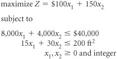
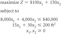
| The branch and bound method is not a solution technique specifically limited to integer programming problems. It is a solution approach that can be applied to a number of different types of problems. The branch and bound approach is based on the principle that the total set of feasible solutions can be partitioned into smaller subsets of solutions. These smaller subsets can then be evaluated systematically until the best solution is found. When the branch and bound approach is applied to an integer programming problem, it is used in conjunction with the normal noninteger solution approach. We will demonstrate the branch and bound method using the following example. The branch and bound method is a solution approach that partitions the feasible solution space into smaller subsets of solutions . The owner of a machine shop is planning to expand by purchasing some new machinespresses and lathes. The owner has estimated that each press purchased will increase profit by $100 per day and each lathe will increase profit by $150 daily. The number of machines the owner can purchase is limited by the cost of the machines and the available floor space in the shop. The machine purchase prices and space requirements are as follows .
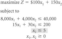
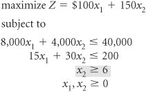
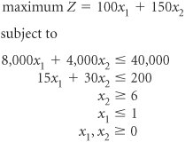
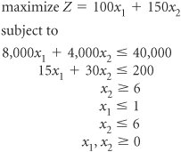
The owner has a budget of $40,000 for purchasing machines and 200 square feet of available floor space. The owner wants to know how many of each type of machine to purchase to maximize the daily increase in profit. The linear programming model for an integer programming problem is formulated in exactly the same way as the linear programming examples in chapters 2 and 4 of the text. The only difference is that in this problem, the decision variables are restricted to integer values because the owner cannot purchase a fraction, or portion, of a machine. The linear programming model follows. where
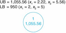
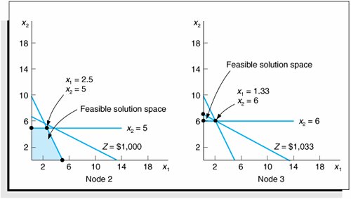
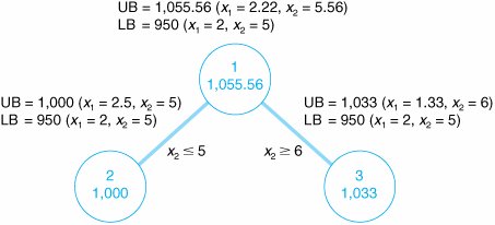
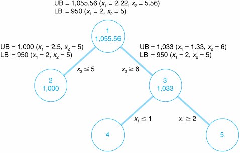
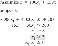
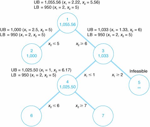
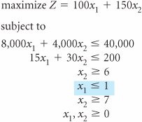
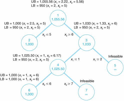
The decision variables in this model are restricted to whole machines. The fact that both decision variables, x 1 and x 2 , can assume any integer value greater than or equal to zero is what gives this model its designation as a total integer model. We begin the branch and bound method by first solving the problem as a regular linear programming model without integer restrictions (i.e., the integer restrictions are relaxed ). The linear programming model for the problem and the optimal relaxed solution is and x 1 = 2.22, x 2 = 5.56, and Z = 1,055.56 A linear programming model solution with no integer restrictions is called a relaxed solution . The branch and bound method employs a diagram consisting of nodes and branches as a framework for the solution process. The first node of the branch and bound diagram, shown in Figure C-1 contains the relaxed linear programming solution shown earlier and the rounded-down solution. Figure C-1. The initial node in the branch and bound diagram The branch and bound method uses a tree diagram of nodes and branches to organize the solution partitioning . Notice that this node has two designated bounds: an upper bound (UB) of $1,055.56 and a lower bound (LB) of $950. The lower bound is the Z value for the rounded-down solution, x 1 = 2 and x 2 = 5; the upper bound is the Z value for the relaxed solution, x 1 = 2.22 and x 2 = 5.56. The optimal integer solution will be between these two bounds. The optimal integer solution will always be between the upper bound of the relaxed solution and a lower bound of the roundeddown integer solution . Rounding down might result in a suboptimal solution. In other words, we are hoping that a Z value greater than $950 might be possible. We are not concerned that a value lower than $950 might be available. Thus, $950 represents a lower bound for our solution. Alternatively, since Z = $1,055.56 reflects an optimal solution point on the solution space boundary , a greater Z value cannot possibly be attained. Hence, Z = $1,055.56 is the upper bound of our solution. Branch on the variable with the solution value with the greatest fractional part . Now that the possible feasible solutions have been narrowed to values between the upper and lower bounds, we must test the solutions within these bounds to determine the best one. The first step in the branch and bound method is to create two solution subsets from the present relaxed solution. This is accomplished by observing the relaxed solution value for each variable, x 1 = 2.22 x 2 = 5.56 and seeing which one is the farthest from the rounded-down integer value (i.e., which variable has the greatest fractional part). The .56 portion of 5.56 is the greatest fractional part; thus, x 2 will be the variable that we will "branch" on. Because x 2 must be an integer value in the optimal solution, the following constraints can be developed. x 2 x 2 Create two constraints (or subsets) to eliminate the fractional part of the solution value In other words, x 2 can be 0, 1, 2, 3, 4, 5, or 6, 7, 8, etc., but it cannot be a value between 5 and 6, such as 5.56. These two new constraints represent the two solution subsets for our solution approach. Each of these constraints will be added to our linear programming model, which will then be solved normally to determine a relaxed solution. This sequence of events is shown on the branch and bound diagram in Figure C-2. The solutions at nodes 2 and 3 will be the relaxed solutions obtained by solving our example model with the appropriate constraints added. Figure C-2. Solution subsets x 2 First, the solution at node 2 is found by solving the following model with the constraint x 2 The optimal solution for this model with integer restrictions relaxed (solved using the computer) is x 1 = 2.5, x 2 = 5, and Z = 1,000. Next, the solution at node 3 is found by solving the model with x 2 The optimal solution for this model with integer restrictions relaxed is x 1 = 1.33, x 2 = 6, and Z = 1,033.33. These solutions with x 2 Figure C-3. Feasible solution spaces for nodes 2 and 3 Notice that in the node 2 graph in Figure C-3, the solution point x 1 = 2.5, x 2 = 5 results in a maximum Z value of $1,000, which is the upper bound for this node. Next, notice that in the node 3 graph, the solution point x 1 = 1.33, x 2 = 6 results in a maximum Z value of $1,033. Thus, $1,033 is the upper bound for node 3. The lower bound at each of these nodes is the maximum integer solution. Since neither of these relaxed solutions is totally integer, the lower bound remains $950, the integer solution value already obtained at node 1 for the rounded-down integer solution. The diagram in Figure C-4 reflects the addition of the upper and lower bounds at each node. Figure C-4. Branch and bound diagram with upper and lower bounds at nodes 2 and 3 Since we do not have an optimal and feasible integer solution yet, we must continue to branch (i.e., partition) the model, from either node 2 or node 3. A look at Figure C-4 reveals that if we branch from node 2, the maximum value that can possibly be achieved is $1,000 (the upper bound). However, if we branch from node 3, a higher maximum value of $1,033 is possible. Thus, we will branch from node 3. In general, always branch from the node with the maximum upper bound . Now the steps for branching previously followed at node 1 are repeated at node 3. First, the variable that has the value with the greatest fractional part is selected. Because x 2 has an integer value, x 1 , with a fractional part of .33, is the only variable we can select. Thus, two new constraints are developed for x 1 , x 1 x 1 This process creates the new branch and bound diagram shown in Figure C-5. Figure C-5. Solution subsets for x 1 Next, the relaxed linear programming model with the new constraints added must be solved at nodes 4 and 5. (However, do not forget that the model is not the original, but the original with the constraint previously added, x 2 The optimal solution for this model with integer restrictions relaxed is x 1 = 1, x 2 = 6.17, and Z = 1,025. Next, consider the node 5 model. However, there is no feasible solution for this model. Therefore, no solution exists at node 5, and we have only to evaluate the solution at node 4. The branch and bound diagram reflecting these results is shown in Figure C-6. Figure C-6. Branch and bound diagram with upper and lower bounds at nodes 4 and 5 The branch and bound diagram in Figure C-6 indicates that we still have not reached an optimal integer solution; thus, we must repeat the branching steps followed earlier. Since a solution does not exist at node 5, there is no comparison between the upper bounds at nodes 4 and 5. Comparing nodes 2 and 4, we must branch from node 4 because it has the greater upper bound. Next, since x 1 has an integer value, x 2 , with a fractional part of .17, is selected by default. The two new constraints developed for x 2 are x 2 x 2 This creates the new branch and bound diagram in Figure C-7. Figure C-7. Solution subsets for x 2 The relaxed linear programming model with the new constraints added must be solved at nodes 6 and 7. Consider the node 6 model first. The optimal solution for this relaxed linear programming model is x 1 = 1, x 2 = 6, and Z = 1,000. Next, consider the node 7 model. However, the solution to this model is infeasible and no solution exists at node 7. The branch and bound diagram reflecting these results is shown in Figure C-8. This version of the branch and bound diagram indicates that the optimal integer solution, x 1 = 1, x 2 = 6, has been reached at node 6. The value of 1,000 at node 6 is the maximum, or upper bound, integer value that can be obtained. It is also the recomputed lower bound because it is the maximum integer solution achieved to this point. Thus, it is not possible to achieve any higher value by further branching from node 6. A comparison of the node 6 solution with those at nodes 2, 5, and 7 shows that a better solution is not possible. The upper bound at node 2 is 1,000, which is the same as that obtained at node 6; thus, node 2 can result in no improvement. The solutions at nodes 5 and 7 are infeasible (and thus further branching will result in only infeasible solutions). By the process of elimination , the integer solution at node 6 is optimal. Figure C-8. The branch and bound diagram with optimal solution at node 6 An optimal integer solution is reached when a feasible integer solution is achieved at a node that has an upper bound greater than or equal to the upper bound at any other ending node . In general, the optimal integer solution is reached when a feasible integer solution is generated at a node and the upper bound at that node is greater than or equal to the upper bound at any other ending node (i.e., a node at the end of a branch). In the context of the original example, this solution indicates that if the machine shop owner purchases one press and six lathes, a daily increase in profit of $1,000 will result. The steps of the branch and bound method for determining an optimal integer solution for a maximization model (with The steps of the branch and bound method .
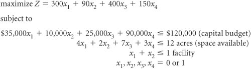
For a minimization model, relaxed solutions are rounded up, and upper and lower bounds are reversed . The branch and bound method can be used for mixed integer problems, except only variables with integer restrictions are rounded down to achieve the initial lower bound and only integer variables are branched on . Solution of the Mixed Integer ModelMixed integer linear programming problems can also be solved using the branch and bound method. The same basic steps that were applied to the total integer model in the previous section are used for a mixed integer model with only a few differences. First, at node 1 only those variables with integer restrictions are rounded down to achieve the lower bound . Second, in determining which variable to branch from, we select the greatest fractional part from among only those variables that must be integer. All other steps remain the same. The optimal solution is reached when a feasible solution is generated at a node that has integer values for those variables requiring integers and that has reached the maximum upper bound of all ending nodes. Solution of the 01 Integer Model The 01 integer model can also be solved using the branch and bound method. First, the 01 restrictions for variables must be reflected as model constraints, x j A community council must decide which recreation facilities to construct in its community. Four new recreation facilities have been proposeda swimming pool, a tennis center, an athletic field, and a gymnasium. The council wants to construct facilities that will maximize the expected daily usage by the residents of the community subject to land and cost limitations. The expected daily usage and cost and land requirements for each facility follow.
The community has a $120,000 construction budget and 12 acres of land. Because the swimming pool and tennis center must be built on the same part of the land parcel , however, only one of these two facilities can be constructed . The council wants to know which of the recreation facilities to construct in order to maximize the expected daily usage. The model for this problem is formulated as follows. where
In this model, the decision variables can have a solution value of either zero or one . If a facility is not selected for construction, the decision variable representing it will have a value of zero. If a facility is selected, its decision variable will have a value of one. The last constraint, x 1 + x 2 To apply the branch and bound method, the following four constraints have to be added to the model in place of the single restriction x 1 , x 2 , x 3 , x 4 = 0 or 1. x 1 x 2 x 3 x 4 The branch and bound method can be used for 01 integer problems by adding " The only other change in the normal branch and bound method is at step 3. Once the variable x j with the greatest fractional part has been determined, the two new constraints developed from this variable are x j = 0 and x j = 1. These two new constraints will form the two branches at each node. Another method for solving 01 integer problems is implicit enumeration . In implicit enumeration, obviously infeasible solutions are eliminated and the remaining solutions are evaluated (i.e., enumerated) to see which is the best. This approach will be demonstrated using our original 01 example model for selecting a recreational facility (i.e., without the x j In implicit enumeration all feasible solutions are evaluated to see which is best . The complete enumeration (i.e., the list of all possible solution sets) for this model is as follows.
Solutions 6, 12, 14, and 16 can be immediately eliminated because they violate the third constraint, x 1 + x 2 The process of eliminating infeasible solutions and then evaluating the feasible solutions to see which is best is the basic principle behind implicit enumeration. However, implicit enumeration is usually done more systematically, by evaluating solutions with branching diagrams like those used in the branch and bound method, rather than by sorting through a complete enumeration as in this previous example. |
 5
5  6
6 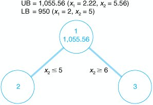


EAN: 2147483647
Pages: 358