Category list

Continuous Probability Distributions

[Page 627 ( continued )]

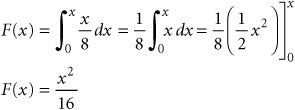
Continuous Probability Distributions

In the first example in this chapter, ComputerWorld's store manager considered a probability distribution of discrete demand values. In the queuing example, the probability distributions were for discrete interarrival times and service times. However, applications of simulation models reflecting continuous distributions are more common than those of models employing discrete distributions.

We have concentrated on examples with discrete distributions because with a discrete distribution, the ranges of random numbers can be explicitly determined and are thus easier to illustrate . When random numbers are being selected according to a continuous probability distribution, a continuous function must be used. For example, consider the following continuous probability function, f ( x ), for time (minutes), x :

The area under the curve, f ( x ), represents the probability of the occurrence of the random variable x . Therefore, the area under the curve must equal 1.0 because the sum of all probabilities of the occurrence of a random variable must equal 1.0. By computing the area under the curve from 0 to any value of the random variable x , we can determine the cumulative probability of that value of x , as follows :

Cumulative probabilities are analogous to the discrete ranges of random numbers we used in previous examples. Thus, we let this function, F ( x ), equal the random number, r ,

[Page 628]

and solve for x ,

By generating a random number, r , and substituting it into this function, we determine a value for x , "time." (However, for a continuous function, the range of random numbers must be between zero and one to correspond to probabilities between 0.0 and 1.00.) For example, if r = .25, then

The purpose of briefly presenting this example is to demonstrate the difference between discrete and continuous functions. This continuous function is relatively simple; as functions become more complex, it becomes more difficult to develop the equation for determining the random variable x from r . Even this simple example required some calculus, and developing more complex models would require a higher level of mathematics.

Simulation of a Machine Breakdown and Maintenance System

In this example we will demonstrate the use of a continuous probability distribution. The Bigelow Manufacturing Company produces a product on a number of machines. The elapsed time between breakdowns of the machines is defined by the following continuous probability distribution:

where

x = weeks between machine breakdowns

A continuous probability distribution of the time between machine breakdowns .

As indicated in the previous section on continuous probability distributions, the equation for generating x , given the random number r ₁ , is

When a machine breaks down, it must be repaired, and it takes either 1, 2, or 3 days for the repair to be completed, according to the discrete probability distribution shown in Table 14.8. Every time a machine breaks down, the cost to the company is an estimated $2,000 per day in lost production until the machine is repaired.

Table 14.8. Probability distribution of machine repair time

Machine Repair Time, y (days)	Probability of Repair Time, P ( y )	Cumulative Probability	Random Number Range, r ₂
1	.15	.15	0.00.15
2	.55	.70	.16.70
3	.30	1.00	.711.00

The company would like to know whether it should implement a machine maintenance program at a cost of $20,000 per year that would reduce the frequency of breakdowns and thus the time for repair. The maintenance program would result in the following continuous probability function for time between breakdowns:

f ( x ) = x /18, 0 x 6 weeks

where

x = weeks between machine breakdowns

[Page 629]

The equation for generating x , given the random number r ₁ , for this probability distribution is

The reduced repair time resulting from the maintenance program is defined by the discrete probability distribution shown in Table 14.9.

Table 14.9. Revised probability distribution of machine repair time with the maintenance program

Machine Repair Time, y (days)	Probability of Repair Time, P ( y )	Cumulative Probability	Random Number Range, r ₂
1	.40	.40	0.00.40
2	.50	.90	.41.90
3	.10	1.00	.911.00

To solve this problem, we must first simulate the existing system to determine an estimate of the average annual repair costs. Then we must simulate the system with the maintenance program installed to see what the average annual repair costs will be with the maintenance program. We will then compare the average annual repair cost with and without the maintenance program and compute the difference, which will be the average annual savings in repair costs with the maintenance program. If this savings is more than the annual cost of the maintenance program ($20,000), we will recommend that it be implemented; if it is less, we will recommend that it not be implemented.

First, we will manually simulate the existing breakdown and repair system without the maintenance program, to see how the simulation model is developed. Table 14.10 illustrates the simulation of machine breakdowns and repair for 20 breakdowns, which occur over a period of approximately 1 year (i.e., 52 weeks).

Table 14.10. Simulation of machine breakdowns and repair times

Breakdowns	r ₁	Time Between Breakdowns, x (weeks)	r ₂	Repair Time, y (days)	Cost, $2,000 y	Cumulative Time, S x (weeks)
1	.45	2.68	.19	2	$ 4,000	2.68
2	.90	3.80	.65	2	4,000	6.48
3	.84	3.67	.51	2	4,000	10.15
4	.17	1.65	.17	2	4,000	11.80
5	.74	3.44	.63	2	4,000	15.24
6	.94	3.88	.85	3	6,000	19.12
7	.07	1.06	.37	2	4,000	20.18
8	.15	1.55	.89	3	6,000	21.73
9	.04	0.80	.76	3	6,000	22.53
10	.31	2.23	.71	3	6,000	24.76
11	.07	1.06	.34	2	4,000	25.82
12	.99	3.98	.11	1	2,000	29.80
13	.97	3.94	.27	2	4,000	33.74
14	.73	3.42	.10	1	2,000	37.16
15	.13	1.44	.59	2	4,000	38.60
16	.03	0.70	.87	3	6,000	39.30
17	.62	3.15	.08	1	2,000	42.45
18	.47	2.74	.08	1	2,000	45.19
19	.99	3.98	.89	3	6,000	49.17
20	.75	3.46	.42	2	4,000	52.63
					$84,000

[Page 630]

The simulation in Table 14.10 results in a total annual repair cost of $84,000. However, this is for only 1 year, and thus it is probably not very accurate.

The next step in our simulation analysis is to simulate the machine breakdown and repair system with the maintenance program installed. We will use the revised continuous probability distribution for time between breakdowns and the revised discrete probability distribution for repair time shown in Table 14.9. Table 14.11 illustrates the manual simulation of machine breakdowns and repair for 1 year.

Table 14.11. Simulation of machine breakdowns and repair with the maintenance program

Breakdowns	r ₁	Time Between Breakdowns, x (weeks)	r ₂	Repair Time, y (days)	Cost, $2,000 y	Cumulative Time, S x (weeks)
1	.45	4.03	.19	1	$ 2,000	4.03
2	.90	5.69	.65	2	4,000	9.72
3	.84	5.50	.51	2	4,000	15.22
4	.17	2.47	.17	1	2,000	17.69
5	.74	5.16	.63	2	4,000	22.85
6	.94	5.82	.85	2	4,000	28.67
7	.07	1.59	.37	1	2,000	30.29
8	.15	2.32	.89	2	4,000	32.58
9	.04	1.20	.76	2	4,000	33.78
10	.31	3.34	.71	2	4,000	37.12
11	.07	1.59	.34	1	2,000	38.71
12	.99	5.97	.11	1	2,000	44.68
13	.97	5.91	.27	1	2,000	50.59
14	.73	5.12	.10	1	2,000	55.71
					$42,000

{% if main.adsdop %}{% include 'adsenceinline.tpl' %}{% endif %}

Table 14.11 shows that the annual repair cost with the maintenance program totals $42,000. Recall that in the manual simulation shown in Table 14.10, the annual repair cost was $84,000 for the system without the maintenance program. The difference between the two annual repair costs is $84,000 42,000 = $42,000. This figure represents the savings in average annual repair cost with the maintenance program. Because the maintenance program will cost $20,000 per year, it would seem that the recommended decision would be to implement the maintenance program and generate an expected annual savings of $22,000 per year (i.e., $42,000 20,000 = $22,000).

However, let us now concern ourselves with the potential difficulties caused by the fact that we simulated each system (the existing one and the system with the maintenance program) only once . Because the time between breakdowns and the repair times are probabilistic, the simulation results could exhibit significant variation. The only way to be sure of the accuracy of our results is to simulate each system many times and compute an average result. Performing these many simulations manually would obviously require a great deal of time and effort. However, Excel can be used to accomplish the required simulation analysis.

Manual simulation is limited because of the amount of real time required to simulate even one trial .

Computer Simulation of the Machine Breakdown Example Using Excel

Exhibit 14.7 shows the Excel spreadsheet model of the simulation of our original machine breakdown example simulated manually in Table 14.10. The Excel simulation is for 100 breakdowns. The random numbers in C14:C113 are generated using the RAND () function, which was used in our previous Excel examples. The "Time Between Breakdowns" values in column D are developed using the formula for the continuous cumulative probability function, = 4*SQRT(C14) , typed in cell D14 and copied in cells D15:D113 .

[Page 631]

Exhibit 14.7.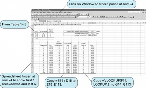

The "Cumulative Time" in column E is computed by copying the formula = E14+D15 in cells E15:E113 . The second stream of random numbers in column F is generated using the RAND () function. The "Repair Time" values in column G are generated from the cumulative probability distribution in the array of cells B6:C8 . As in our previous examples, we name this array "Lookup" and copy the formula = VLOOKUP(F14,Lookup,2 ) in cells G14:G113 . The cost values in column H are computed by entering the formula = 2000*G14 in cell H14 and copying it to cells H15:H113 .

[Page 632]

The "Average Annual Cost" in cell H7 is computed with the formula = SUM(H14:H113 )/( E113/52 ). For this, the original problem, the annual cost is $82,397.35, which is not too different from the manual simulation in Table 14.10.

Exhibit 14.8 shows the Excel spreadsheet simulation for the modified breakdown system with the new maintenance program, which was simulated manually in Table 14.11. The two differences in this simulation model are the cumulative probability distribution formulas for the time between breakdowns and the reduced repair time distributions from Table 14.9 in cells A6:C8 .

Exhibit 14.8.

(This item is displayed on page 631 in the print version)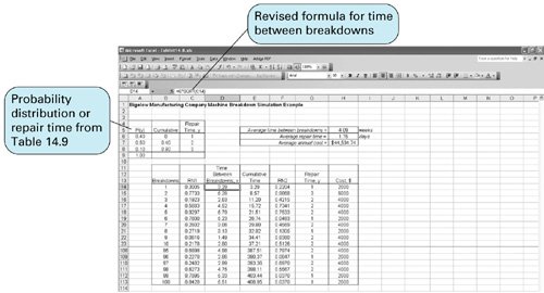

The average annual cost for this model, shown in cell H8, is $44,504.74. This annual cost is only slightly higher than the $42,000 obtained from the manual simulation in Table 14.11. Thus, as before, the decision should be to implement the new maintenance system.