The Single-Server Waiting Line System
| A single server with a single waiting line is the simplest form of queuing system. As such, it will be used to demonstrate the fundamentals of a queuing system. As an example of this kind of system, consider Fast Shop Market. Fast Shop Market has one checkout counter and one employee who operates the cash register at the checkout counter. The combination of the cash register and the operator is the server (or service facility) in this queuing system; the customers who line up at the counter to pay for their selections form the waiting line , or queue . The configuration of this example queuing system is shown in Figure 13.1. Components of a waiting line system include arrivals, servers, and the waiting line structure . Figure 13.1. The Fast Shop Market waiting line system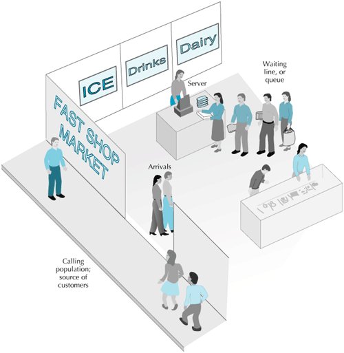 The most important factors to consider in analyzing a queuing system such as the one in Figure 13.1 are the following:
We will discuss each of these items as it relates to our example. The Queue DisciplineThe queue discipline is the order in which waiting customers are served. Customers at Fast Shop Market are served on a "first-come, first-served" basis. That is, the first person in line at the checkout counter is served first. This is the most common type of queue discipline. However, other disciplines are possible. For example, a machine operator might stack in-process parts beside a machine so that the last part is on top of the stack and will be selected first. This queue discipline is referred to as "last-in, first-out." Or the machine operator might simply reach into a box full of parts and select one at random. In this case, the queue discipline is random. Often customers are scheduled for service according to a predetermined appointment, such as patients at a doctor's or dentist's office or diners at a restaurant where reservations are required. In this case, the customers are taken according to a prearranged schedule, regardless of when they arrive at the facility. One final example of the many types of queue disciplines is when customers are processed alphabetically according to their last names , such as at school registration or at job interviews. The queue discipline is the order in which waiting customers are served . The Calling PopulationThe calling population is the source of the customers to the market, which in this case is assumed to be infinite. In other words, there is such a large number of possible customers in the area where the store is located that the number of potential customers is assumed to be infinite. Some queuing systems have finite calling populations. For example, the repair garage of a trucking firm that has 20 trucks has a finite calling population. The queue is the number of trucks waiting to be repaired, and the finite calling population is the 20 trucks . However, queuing systems that have an assumed infinite calling population are more common. The calling population is the source of customers; it may be infinite or finite . The Arrival RateThe arrival rate is the rate at which customers arrive at the service facility during a specified period of time. This rate can be estimated from empirical data derived from studying the system or a similar system, or it can be an average of these empirical data. For example, if 100 customers arrive at a store checkout counter during a 10-hour day, we could say the arrival rate averages 10 customers per hour. However, although we might be able to determine a rate for arrivals by counting the number of paying customers at the market during a 10-hour day, we would not know exactly when these customers would arrive on the premises. In other words, it might be that no customers would arrive during one hour and 20 customers would arrive during another hour . In general, these arrivals are assumed to be independent of each other and to vary randomly over time. The arrival rate is the frequency at which customers arrive at a waiting line according to a probability distribution .
Given these assumptions, it is further assumed that arrivals at a service facility conform to some probability distribution. Although arrivals could be described by any distribution, it has been determined (through years of research and the practical experience of people in the field of queuing) that the number of arrivals per unit of time at a service facility can frequently be defined by a Poisson distribution . (Appendix C at the end of this text contains a more detailed presentation of the Poisson distribution.) The arrival rate ( l ) is most frequently described by a Poisson distribution . The Service RateThe service rate is the average number of customers who can be served during a specified period of time. For our Fast Shop Market example, 30 customers can be checked out (served) in 1 hour. A service rate is similar to an arrival rate in that it is a random variable. In other words, such factors as different sizes of customer purchases, the amount of change the cashier must count out, and different forms of payment alter the number of persons that can be served over time. Again, it is possible that only 10 customers might be checked out during one hour and 40 customers might be checked out during the following hour. The service rate is the average number of customers who can be served during a time period . The description of arrivals in terms of a rate and of service in terms of time is a convention that has developed in queuing theory. Like arrival rate, service time is assumed to be defined by a probability distribution. It has been determined by researchers in the field of queuing that service times can frequently be defined by a negative exponential probability distribution. (Appendix C at the end of this text contains a more detailed presentation of the exponential distribution.) However, to analyze a queuing system, both arrivals and service must be in compatible units of measure. Thus, service time must be expressed as a service rate to correspond with an arrival rate. The service time can often be described by the negative exponential distribution . The Single-Server ModelThe Fast Shop Market checkout counter is an example of a single-server queuing system with the following characteristics:
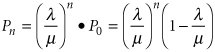
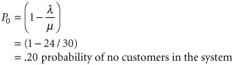
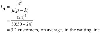
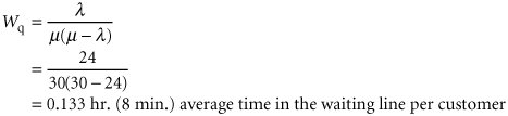
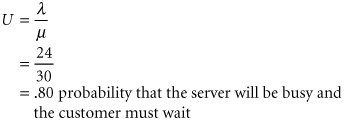
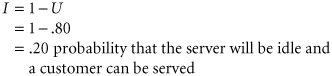
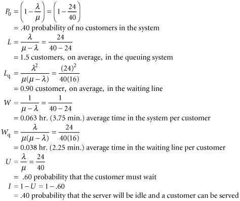
Assumptions of the basic single-server model . These assumptions have been used to develop a model of a single-server queuing system. However, the analytical derivation of even this simplest queuing model is relatively complex and lengthy. Thus, we will refrain from deriving the model in detail and will consider only the resulting queuing formulas. The reader must keep in mind, however, that these formulas are applicable only to queuing systems having the foregoing conditions. Given that l = the arrival rate (average number of arrivals per time period) µ = the service rate (average number served per time period) l = mean arrival rate; µ = mean service rate . and that l < µ (customers are served at a faster rate than they arrive), we can state the following formulas for the operating characteristics of a single-server model. Customers must be served faster than they arrive, or an infinitely large queue will build up . The probability that no customers are in the queuing system (either in the queue or being served) is Basic single-server queuing formulas . The probability that n customers are in the queuing system is The average number of customers in the queuing system (i.e., the customers being serviced and in the waiting line) is The average number of customers in the waiting line is The average time a customer spends in the total queuing system (i.e., waiting and being served) is The average time a customer spends waiting in the queue to be served is The probability that the server is busy (i.e., the probability that a customer has to wait), known as the utilization factor , is The probability that the server is idle (i.e., the probability that a customer can be served) is This last term , 1 ( l / µ), is also equal to P . That is, the probability of no customers in the queuing system is the same as the probability that the server is idle. We can compute these various operating characteristics for Fast Shop Market by simply substituting the average arrival and service rates into the foregoing formulas. For example, if l = 24 customers per hour arrive at checkout counter µ = 30 customers per hour can be checked out then Several important aspects of both the general model and this particular example will now be discussed in greater detail. Queuing system operating statistics are steady state , or constant, over time . First, the operating characteristics are averages. Also, they are assumed to be steady-state averages. Steady state is a constant average level that a system realizes after a period of time. For a queuing system, the steady state is represented by the average operating statistics, also determined over a period of time. Related to this condition is the fact that the utilization factor, U , must be less than one: U < 1 or and l < m In other words, the ratio of the arrival rate to the service rate must be less than one, which also means the service rate must be greater than the arrival rate if this model is to be used. The server must be able to serve customers faster than they come into the store in the long run, or the waiting line will grow to an infinite size , and the system will never reach a steady state. The Effect of Operating Characteristics on Managerial DecisionsNow let us consider the operating characteristics of our example as they relate to management decisions. The arrival rate of 24 customers per hour means that, on average, a customer arrives every 2.5 minutes (i.e., 1/24 x 60 minutes). This indicates that the store is very busy. Because of the nature of the store, customers purchase few items and expect quick service. Customers expect to spend a relatively large amount of time in a supermarket because typically they make larger purchases. But customers who shop at a convenience market do so, at least in part, because it is quicker than a supermarket . Given customers' expectations, the store's manager believes that it is unacceptable for a customer to wait 8 minutes and spend a total of 10 minutes in the queuing system (not including the actual shopping time). The manager wants to test several alternatives for reducing customer waiting time: (1) the addition of another employee to pack up the purchases and (2) the addition of a new checkout counter. Alternative I: The Addition of an Employee The addition of an extra employee will cost the store manager $150 per week. With the help of the national office's marketing research group , the manager has determined that for each minute that average customer waiting time is reduced, the store avoids a loss in sales of $75 per week. (That is, the store loses money when customers leave prior to shopping because of the long line or when customers do not return.) If a new employee is hired , customers can be served in less time. In other words, the service rate, which is the number of customers served per time period, will increase . The previous service rate was µ = 30 customers served per hour The addition of a new employee will increase the service rate to µ = 40 customers served per hour It will be assumed that the arrival rate will remain the same ( l = 24 per hour) because the increased service rate will not increase arrivals but instead will minimize the loss of customers. (However, it is not illogical to assume that an increase in service might increase arrivals in the long run.) Given the new l and µ values, the operating characteristics can be recomputed as follows : Remember that these operating characteristics are averages that result over a period of time; they are not absolutes. In other words, customers who arrive at the Fast Shop Market checkout counter will not find 0.90 customer in line. There could be no customers, or one, two, or three customers, for example. The value 0.90 is simply an average that occurs over time, as do the other operating characteristics. The average waiting time per customer has been reduced from 8 minutes to 2.25 minutes, a significant amount. The savings (that is, the decrease in lost sales) is computed as follows: 8.00 min. 2.25 min. = 5.75 min. 5.75 min. x $75/min. = $431.25 Because the extra employee costs management $150 per week, the total savings will be $431.25 $150 = $281.25 per week The store manager would probably welcome this savings and consider the preceding operating statistics preferable to the previous ones for the condition where the store had only one employee. Alternative II: The Addition of a New Checkout Counter Next we will consider the manager's alternative of constructing a new checkout counter. The total cost of this project would be $6,000, plus an extra $200 per week for an additional cashier. The new checkout counter would be opposite the present counter (so that the servers would have their backs to each other in an enclosed counter area). There would be several display cases and racks between the two lines so that customers waiting in line would not move back and forth between the lines. (Such movement, called jockeying , would invalidate the queuing formulas we already developed.) We will assume that the customers would divide themselves equally between the two lines, so the arrival rate for each line would be half of the prior arrival rate for a single checkout counter. Thus, the new arrival rate for each checkout counter is l = 12 customers per hour and the service rate remains the same for each of the counters: µ = 30 customers served per hour Substituting this new arrival rate and the service rate into our queuing formulas results in the following operating characteristics:
Using the same sales savings of $75 per week for each minute's reduction in waiting time, we find that the store would save
Next we subtract the $200 per week cost for the new cashier from this amount saved: $500 200 = $300 Because the capital outlay of this project is $6,000, it would take 20 weeks ($6,000/$300 = 20 weeks) to recoup the initial cost (ignoring the possibility of interest on the $6,000). Once the cost has been recovered, the store would save $18.75 ($300.00 281.25) more per week by adding a new checkout counter rather than simply hiring an extra employee. However, we must not disregard the fact that during the 20-week cost recovery period, the $281.25 savings incurred by simply hiring a new employee would be lost. Table 13.1 presents a summary of the operating characteristics for each alternative. For the store manager, both of these alternatives seem preferable to the original conditions, which resulted in a lengthy waiting time of 8 minutes per customer. However, the manager might have a difficult time selecting between the two alternatives. It might be appropriate to consider other factors besides waiting time. For example, employee idle time is .40 with the first alternative and .60 with the second, which seems to be a significant difference. An additional factor is the loss of space resulting from a new checkout counter. Table 13.1. Operating characteristics for each alternative system
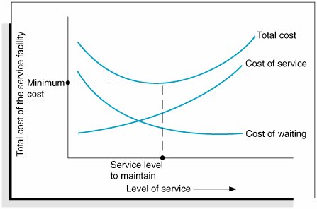
However, the final decision must be based on the manager's own experience and perceived needs. As we have noted previously, the results of queuing analysis provide information for decision making but do not result in an actual recommended decision, as an optimization model would. Our two example alternatives illustrate the cost trade-offs associated with improved service. As the level of service increases, the corresponding cost of this service also increases. For example, when we added an extra employee in alternative I, the service was improved, and the cost of providing service also increased. But when the level of service was increased, the costs associated with customer waiting decreased. Maintaining an appropriate level of service should minimize the sum of these two costs as much as possible. This cost trade-off relationship is summarized in Figure 13.2. As the level of service increases , the cost of service goes up and the waiting cost goes down. The sum of these costs results in a total cost curve, and the level of service that should be maintained is the level where this total cost curve is at a minimum. (However, this does not mean we can determine an exact optimal minimum cost solution because the service and waiting characteristics we can determine are averages and thus uncertain .) Figure 13.2. Cost trade-off for service levels As the level of service improves , the cost of service increases . Computer Solution of the Single-Server Model with Excel and Excel QMExcel spreadsheets can be used to solve queuing problems, although someone must enter all the queuing formulas into spreadsheet cells. Exhibit 13.1 shows a spreadsheet set up to solve the single-server model for the original Fast Shop Market example. Notice that the arrival rate is entered in cell D3, the service rate is entered in cell D4, and our single-server model queuing formulas are entered in cells D6 to D10. For example, cell D7 includes the formula for L q , average number of customers in the system, shown on the formula bar at the top of the spreadsheet. Exhibit 13.1.(This item is displayed on page 582 in the print version)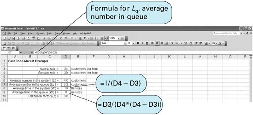
Excel QM includes a spreadsheet macro for waiting line (i.e., queuing) analysis. Excel QM includes all the different queuing models that will be presented in this chapter. The queuing macro in Excel QM is one of the more useful ones in this text because some of the queuing formulas we will introduce are complex and often difficult to set up manually in spreadsheet cells. After Excel QM has been activated, the "Waiting Line Analysis" menu is accessed from the "QM" menu on the menu bar at the top of the spreadsheet. This will result in a Spreadsheet Initialization window, which will enable us to title the problem and specify some of the spreadsheet output. Exhibit 13.2 shows the Excel QM spreadsheet for our Fast Shop Market single-server model. When this spreadsheet first appears, cells B7:B8 contain example data values, and the results relate to these arrival and service rates. Thus, the first step is to enter the arrival and service rates for our Fast Shop Market example in cells B7:B8 . The results will be computed automatically, using the queuing formulas already embedded in the macro. Exhibit 13.2.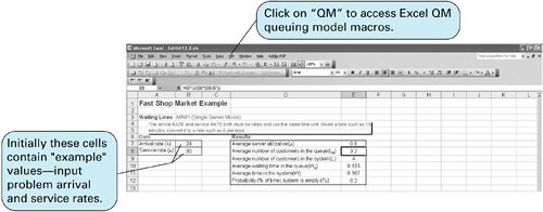 Computer Solution of the Single-Server Model with QM for WindowsQM for Windows has a module that is capable of performing queuing analysis. As an illustration of the computerized analysis of the single-server queuing system, we will use QM for Windows to analyze the Fast Shop Market example. The model input and solution output are shown in Exhibit 13.3. Exhibit 13.3.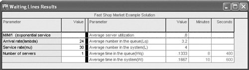 |


EAN: 2147483647
Pages: 358