Decision Making with Probabilities
| The decision-making criteria just presented were based on the assumption that no information regarding the likelihood of the states of nature was available. Thus, no probabilities of occurrence were assigned to the states of nature, except in the case of the equal likelihood criterion. In that case, by assuming that each state of nature was equally likely and assigning a weight of .50 to each state of nature in our example, we were implicitly assigning a probability of .50 to the occurrence of each state of nature. It is often possible for the decision maker to know enough about the future states of nature to assign probabilities to their occurrence. Given that probabilities can be assigned, several decision criteria are available to aid the decision maker. We will consider two of these criteria: expected value and expected opportunity loss (although several others, including the maximum likelihood criterion , are available). Expected ValueTo apply the concept of expected value as a decision-making criterion, the decision maker must first estimate the probability of occurrence of each state of nature. Once these estimates have been made, the expected value for each decision alternative can be computed. The expected value is computed by multiplying each outcome (of a decision) by the probability of its occurrence and then summing these products. The expected value of a random variable x , written symbolically as E ( x ), is computed as follows : where n = number of values of the random variable x Expected value is computed by multiplying each decision outcome under each state of nature by the probability of its occurrence . Using our real estate investment example, let us suppose that, based on several economic forecasts, the investor is able to estimate a .60 probability that good economic conditions will prevail and a .40 probability that poor economic conditions will prevail. This new information is shown in Table 12.7. Table 12.7. Payoff table with probabilities for states of nature
The expected value ( E V) for each decision is computed as follows:
The best decision is the one with the greatest expected value. Because the greatest expected value is $44,000, the best decision is to purchase the office building. This does not mean that $44,000 will result if the investor purchases the office building; rather, it is assumed that one of the payoff values will result (either $100,000 or $40,000). The expected value means that if this decision situation occurred a large number of times, an average payoff of $44,000 would result. Alternatively, if the payoffs were in terms of costs, the best decision would be the one with the lowest expected value. Expected Opportunity LossA decision criterion closely related to expected value is expected opportunity loss . To use this criterion, we multiply the probabilities by the regret (i.e., opportunity loss) for each decision outcome rather than multiplying the decision outcomes by the probabilities of their occurrence, as we did for expected monetary value. Expected opportunity loss is the expected value of the regret for each decision . The concept of regret was introduced in our discussion of the minimax regret criterion. The regret values for each decision outcome in our example were shown in Table 12.6. These values are repeated in Table 12.8, with the addition of the probabilities of occurrence for each state of nature. Table 12.8. Regret (opportunity loss) table with probabilities for states of nature
The expected opportunity loss ( EOL ) for each decision is computed as follows:
As with the minimax regret criterion, the best decision results from minimizing the regret, or, in this case, minimizing the expected regret or opportunity loss. Because $28,000 is the minimum expected regret, the decision is to purchase the office building. The expected value and expected opportunity loss criteria result in the same decision . Notice that the decisions recommended by the expected value and expected opportunity loss criteria were the sameto purchase the office building. This is not a coincidence because these two methods always result in the same decision. Thus, it is repetitious to apply both methods to a decision situation when one of the two will suffice. In addition, note that the decisions from the expected value and expected opportunity loss criteria are totally dependent on the probability estimates determined by the decision maker. Thus, if inaccurate probabilities are used, erroneous decisions will result. It is therefore important that the decision maker be as accurate as possible in determining the probability of each state of nature. Solution of Expected Value Problems with QM for WindowsQM for Windows not only solves decision analysis problems without probabilities but also has the capability to solve problems using the expected value criterion. A summary of the input data and the solution output for our real estate example is shown in Exhibit 12.5. Notice that the expected value results are included in the third column of this solution screen. Exhibit 12.5.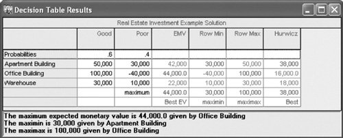 Solution of Expected Value Problems with Excel and Excel QMThis type of expected value problem can also be solved by using an Excel spreadsheet. Exhibit 12.6 shows our real estate investment example set up in a spreadsheet format. Cells E7, E8, and E9 include the expected value formulas for this example. The expected value formula for the first decision, purchasing the apartment building, is embedded in cell E7 and is shown on the formula bar at the top of the spreadsheet. Exhibit 12.6. Excel QM is a set of spreadsheet macros that is included on the CD that accompanies this text, and it has a macro to solve decision analysis problems. Once activated, Excel QM is accessed by clicking on "QM" on the menu bar at the top of the spreadsheet. Clicking on "Decision Analysis" will result in a Spreadsheet Initialization window. After entering several problem parameters, including the number of decisions and states of nature, and then clicking on "OK," the spreadsheet shown in Exhibit 12.7 will result. Initially, this spreadsheet contains example values in cells B8:C11 . Exhibit 12.7 shows the spreadsheet with our problem data already typed in. The results are computed automatically as the data are entered, using the cell formulas already embedded in the macro. Exhibit 12.7. Expected Value of Perfect InformationIt is often possible to purchase additional information regarding future events and thus make a better decision. For example, a real estate investor could hire an economic forecaster to perform an analysis of the economy to more accurately determine which economic condition will occur in the future. However, the investor (or any decision maker) would be foolish to pay more for this information than he or she stands to gain in extra profit from having the information. That is, the information has some maximum value that represents the limit of what the decision maker would be willing to spend . This value of information can be computed as an expected valuehence its name , the expected value of perfect information (also referred to as EVPI) . The expected value of perfect information is the maximum amount a decision maker would pay for additional information . To compute the expected value of perfect information, we first look at the decisions under each state of nature. If we could obtain information that assured us which state of nature was going to occur (i.e., perfect information), we could select the best decision for that state of nature. For example, in our real estate investment example, if we know for sure that good economic conditions will prevail, then we will decide to purchase the office building. Similarly, if we know for sure that poor economic conditions will occur, then we will decide to purchase the apartment building. These hypothetical "perfect" decisions are summarized in Table 12.9. Table 12.9. Payoff table with decisions, given perfect information
The probabilities of each state of nature (i.e., .60 and .40) tell us that good economic conditions will prevail 60% of the time and poor economic conditions will prevail 40% of the time (if this decision situation is repeated many times). In other words, even though perfect information enables the investor to make the right decision, each state of nature will occur only a certain portion of the time. Thus, each of the decision outcomes obtained using perfect information must be weighted by its respective probability: $100,000(.60) + 30,000(.40) = $72,000 The amount $72,000 is the expected value of the decision, given perfect information, not the expected value of perfect information. The expected value of perfect information is the maximum amount that would be paid to gain information that would result in a decision better than the one made without perfect information. Recall that the expected value decision without perfect information was to purchase an office building, and the expected value was computed as EV (office) = $100,000(.60) 40,000(.40) = $44,000 The expected value of perfect information is computed by subtracting the expected value without perfect information ($44,000) from the expected value given perfect information ($72,000): EVPI = $72,000 44,000 = $28,000 EVPI equals the expected value, given perfect information, minus the expected value without perfect information . The expected value of perfect information, $28,000, is the maximum amount that the investor would pay to purchase perfect information from some other source, such as an economic forecaster. Of course, perfect information is rare and usually unobtainable. Typically, the decision maker would be willing to pay some amount less than $28,000, depending on how accurate (i.e., close to perfection ) the decision maker believes the information is. It is interesting to note that the expected value of perfect information, $28,000 for our example, is the same as the expected opportunity loss (EOL) for the decision selected, using this later criterion: EOL (office) = $0(.60) + 70,000(.40) = $28,000 The expected value of perfect information equals the expected opportunity loss for the best decision . This will always be the case, and logically so, because regret reflects the difference between the best decision under a state of nature and the decision actually made . This is actually the same thing determined by the expected value of perfect information. Excel QM for decision analysis computes the expected value of perfect information, as shown in cell E17 at the bottom of the spreadsheet in Exhibit 12.7. The expected value of perfect information can also be determined by using Excel. Exhibit 12.8 shows the EVPI for our real estate investment example. Exhibit 12.8.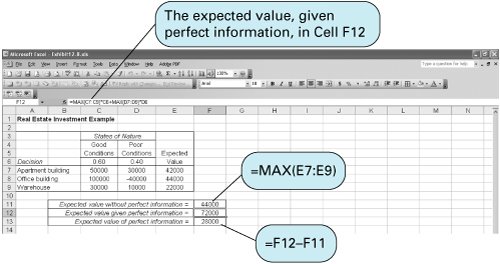 Decision TreesAnother useful technique for analyzing a decision situation is using a decision tree . A decision tree is a graphical diagram consisting of nodes and branches. In a decision tree the user computes the expected value of each outcome and makes a decision based on these expected values. The primary benefit of a decision tree is that it provides an illustration (or picture) of the decision-making process. This makes it easier to correctly compute the necessary expected values and to understand the process of making the decision. A decision tree is a diagram consisting of square decision nodes, circle probability nodes, and branches representing decision alternatives . We will use our example of the real estate investor to demonstrate the fundamentals of decision tree analysis. The various decisions, probabilities, and outcomes of this example, initially presented in Table 12.7, are repeated in Table 12.10. The decision tree for this example is shown in Figure 12.2. Table 12.10. Payoff table for real estate investment example
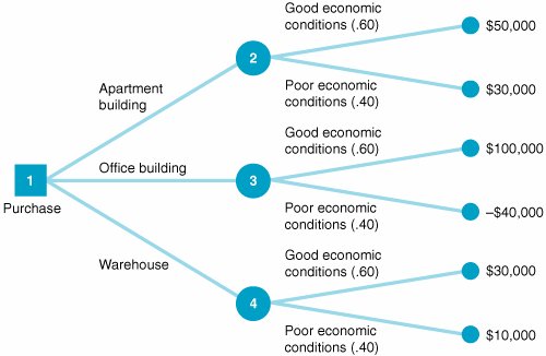
Figure 12.2. Decision tree for real estate investment example The circles ( ) and the square ( The decision tree represents the sequence of events in a decision situation. First, one of the three decision choices is selected at node 1. Depending on the branch selected, the decision maker arrives at probability node 2, 3, or 4, where one of the states of nature will prevail, resulting in one of six possible payoffs. The expected value is computed at each probability node . Determining the best decision by using a decision tree involves computing the expected value at each probability node. This is accomplished by starting with the final outcomes (payoffs) and working backward through the decision tree toward node 1. First, the expected value of the payoffs is computed at each probability node: EV (node 2) = .60($50,000) +.40($30,000) = $42,000 EV (node 3) = .60($100,000) +.40($40,000) = $44,000 EV (node 4) = .60($30,000) +.40($10,000) = $22,000 Branches with the greatest expected value are selected . These values are now shown as the expected payoffs from each of the three branches emanating from node 1 in Figure 12.3. Each of these three expected values at nodes 2, 3, and 4 is the outcome of a possible decision that can occur at node 1. Moving toward node 1, we select the branch that comes from the probability node with the highest expected payoff. In Figure 12.3, the branch corresponding to the highest payoff, $44,000, is from node 1 to node 3. This branch represents the decision to purchase the office building. The decision to purchase the office building, with an expected payoff of $44,000, is the same result we achieved earlier by using the expected value criterion. In fact, when only one decision is to be made (i.e., there is not a series of decisions), the decision tree will always yield the same decision and expected payoff as the expected value criterion. As a result, in these decision situations a decision tree is not very useful. However, when a sequence or series of decisions is required, a decision tree can be very useful. Figure 12.3. Decision tree with expected value at probability nodes Decision Trees with QM for WindowsIn QM for Windows, when the "Decision Analysis" module is accessed and you click on "New" to input a new problem, a menu appears that allows you to select either "Decision Tables" or "Decision Trees." Exhibit 12.9 shows the Decision Tree Results solution screen for our real estate investment example. Notice that QM for Windows requires that all nodes be numbered, including the end, or terminal, nodes, which are shown as solid dots in Figure 12.3. For QM for Windows, we have numbered these end nodes 5 through 10. Exhibit 12.9.(This item is displayed on page 530 in the print version)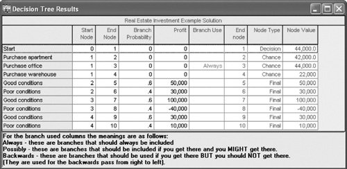 Decision Trees with Excel and TreePlanTreePlan is an Excel add-in program developed by Michael Middleton to construct and solve decision trees in an Excel spreadsheet format. Although Excel has the graphical and computational capability to develop decision trees, it is a difficult and slow process. TreePlan is basically a decision tree template that greatly simplifies the process of setting up a decision tree in Excel. The first step in using TreePlan is to gain access to it. The best way to go about this is to copy the TreePlan add-in file, TreePlan.xla, from the CD accompanying this text onto your hard drive and then add it to the "Tools/Add-Ins" menu that you access at the top of your spreadsheet screen. Once you have added TreePlan to the "Tools" menu, you can invoke it by clicking on the "Decision Trees" menu item. We will demonstrate how to use TreePlan with our real estate investment example shown in Figure 12.3. The first step in using TreePlan is to generate a new tree on which to begin work. Exhibit 12.10 shows a new tree that we generated by positioning the cursor on cell B1 and then invoking the "Tools" menu and clicking on "Decision Trees." This results in a menu from which we click on "New Tree," which creates the decision tree shown in Exhibit 12.10. Exhibit 12.10. The decision tree in Exhibit 12.10 uses the normal nodal convention we used in creating the decision trees in Figures 12.2 and 12.3squares for decision nodes and circles for probability nodes (which TreePlan calls event nodes ). However, this decision tree is only a starting point or template that we need to expand to replicate our example decision tree in Figure 12.3. In Figure 12.3, three branches emanate from the first decision node, reflecting the three investment decisions in our example. To create a third branch using TreePlan, click on the decision node in cell B5 in Exhibit 12.10 and then invoke TreePlan from the "Tools" menu. A window will appear, with several menu items, including "Add Branch." Select this menu item and click on "OK." This will create a third branch on our decision tree, as shown in Exhibit 12.11. Exhibit 12.11. Next we need to expand our decision tree in Exhibit 12.11 by adding probability nodes (2, 3, and 4 in Figure 12.3) and branches from these nodes for our example. To add a new node, click on the end node in cell F3 in Exhibit 12.11 and then invoke TreePlan from the "Tools" menu. From the menu window that appears, select "Change to Event Node" and then select "Two Branches" from the same menu and click on "OK." This process must be repeated two more times for the other two end nodes (in cells F8 and F13) to create our three probability nodes. The resulting decision tree is shown in Exhibit 12.12, with the new probability nodes at cells F5, F15, and F25 and with accompanying branches. Exhibit 12.12.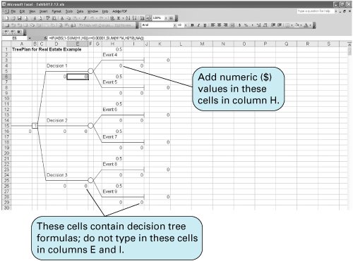 The next step is to edit the decision tree labels and add the numeric data from our example. Generic descriptive labels are shown above each branch in Exhibit 12.12for example, "Decision 1" in cell D4 and "Event 4" in cell H2. We edit the labels the same way we would edit any spreadsheet. For example, if we click on cell D4, we can type in "Apartment Building" in place of "Decision 1," reflecting the decision corresponding to this branch in our example, as shown in Figure 12.3. We can change the other labels on the other branches the same way. The decision tree with the edited labels corresponding to our example is shown in Exhibit 12.13. Exhibit 12.13.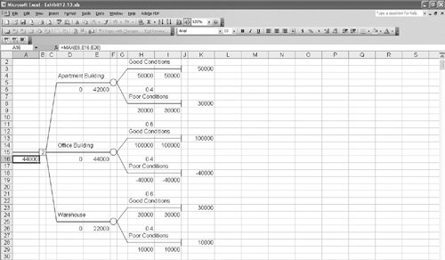 Looking back to Exhibit 12.12 for a moment, focus on the two 0 values below each branchfor example, in cells D6 and E6 and in cells H9 and I4. The first 0 cell is where we type in the numeric value (i.e., $ amount) for that branch. For our example, we would type in 50,000 in cell H4, 30,000 in H9, 100,000 in H14, and so on. These values are shown on the decision tree in Exhibit 12.13. Likewise, we would type in the probabilities for the branches in the cells just above the branchH1, H6, H11, and so on. For example, we would type in 0.60 in cell H1 and 0.40 in cell H6. These probabilities are also shown in Exhibit 12.13. However, we need to be very careful not to type anything into the second 0 branch cellfor example, E6, I4, I9, E16, I14, I19, and so on. These cells automatically contain the decision tree formulas that compute the expected values at each node and select the best decision branches, so we do not want to type anything in these cells that would eliminate these formulas. For example, in Exhibit 12.12 the formula in cell E6 is shown on the formula bar at the top of the screen. This is the expected value for that probability node. The expected value for this decision tree and our example, $44,000, is shown in cell A16 in Exhibit 12.13. Sequential Decision TreesAs noted earlier, when a decision situation requires only a single decision, an expected value payoff table will yield the same result as a decision tree. However, a payoff table is usually limited to a single decision situation, as in our real estate investment example. If a decision situation requires a series of decisions, then a payoff table cannot be created, and a decision tree becomes the best method for decision analysis. A sequential decision tree illustrates a situation requiring a series of decisions To demonstrate the use of a decision tree for a sequence of decisions, we will alter our real estate investment example to encompass a 10-year period during which several decisions must be made. In this new example, the first decision facing the investor is whether to purchase an apartment building or land. If the investor purchases the apartment building, two states of nature are possible: Either the population of the town will grow (with a probability of .60) or the population will not grow (with a probability of .40). Either state of nature will result in a payoff. On the other hand, if the investor chooses to purchase land, 3 years in the future another decision will have to be made regarding the development of the land. The decision tree for this example, shown in Figure 12.4, contains all the pertinent data, including decisions, states of nature, probabilities, and payoffs. Figure 12.4. Sequential decision tree(This item is displayed on page 535 in the print version)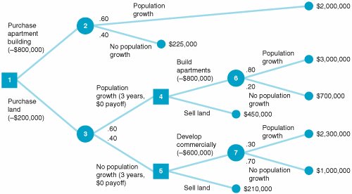
At decision node 1 in Figure 12.4, the decision choices are to purchase an apartment building and to purchase land. Notice that the cost of each venture ($800,000 and $200,000, respectively) is shown in parentheses. If the apartment building is purchased, two states of nature are possible at probability node 2: The town may exhibit population growth, with a probability of .60, or there may be no population growth or a decline, with a probability of .40. If the population grows, the investor will achieve a payoff of $2,000,000 over a 10-year period. (Note that this whole decision situation encompasses a 10-year time span.) However, if no population growth occurs, a payoff of only $225,000 will result. If the decision is to purchase land, two states of nature are possible at probability node 3. These two states of nature and their probabilities are identical to those at node 2; however, the payoffs are different. If population growth occurs for a 3-year period , no payoff will occur, but the investor will make another decision at node 4 regarding development of the land. At that point, either apartments will be built, at a cost of $800,000, or the land will be sold, with a payoff of $450,000. Notice that the decision situation at node 4 can occur only if population growth occurs first. If no population growth occurs at node 3, there is no payoff, and another decision situation becomes necessary at node 5: The land can be developed commercially at a cost of $600,000, or the land can be sold for $210,000. (Notice that the sale of the land results in less profit if there is no population growth than if there is population growth.) If the decision at decision node 4 is to build apartments, two states of nature are possible: The population may grow, with a conditional probability of .80, or there may be no population growth, with a conditional probability of .20. The probability of population growth is higher (and the probability of no growth is lower) than before because there has already been population growth for the first 3 years, as shown by the branch from node 3 to node 4. The payoffs for these two states of nature at the end of the 10-year period are $3,000,000 and $700,000, respectively, as shown in Figure 12.4. If the investor decides to develop the land commercially at node 5, then two states of nature can occur: Population growth can occur, with a probability of .30 and an eventual payoff of $2,300,000, or no population growth can occur, with a probability of .70 and a payoff of $1,000,000. The probability of population growth is low (i.e., .30) because there has already been no population growth, as shown by the branch from node 3 to node 5. This decision situation encompasses several sequential decisions that can be analyzed by using the decision tree approach outlined in our earlier (simpler) example. As before, we start at the end of the decision tree and work backward toward a decision at node 1. First, we must compute the expected values at nodes 6 and 7: EV (node 6) = .80($3,000,000) +.20($700,000) = $2,540,000 EV (node 7) = .30($2,300,000) +.70($1,000,000) = $1,390,000 These expected values (and all other nodal values) are shown in boxes in Figure 12.5. Figure 12.5. Sequential decision tree with nodal expected values(This item is displayed on page 536 in the print version)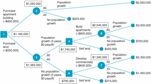 At decision nodes 4 and 5, we must make a decision. As with a normal payoff table, we make the decision that results in the greatest expected value. At node 4 we have a choice between two values: $1,740,000, the value derived by subtracting the cost of building an apartment building ($800,000) from the expected payoff of $2,540,000, or $450,000, the expected value of selling the land computed with a probability of 1.0. The decision is to build the apartment building, and the value at node 4 is $1,740,000. This same process is repeated at node 5. The decisions at node 5 result in payoffs of $790,000 (i.e., $1,390,000 - 600,000 = $790,000) and $210,000. Because the value $790,000 is higher, the decision is to develop the land commercially. Next, we must compute the expected values at nodes 2 and 3: EV (node 2) = .60($2,000,000) +.40($225,000) = $1,290,000 EV (node 3) = .60($1,740,000) +.40($790,000) = $1,360,000 (Note that the expected value for node 3 is computed from the decision values previously determined at nodes 4 and 5.) Now we must make the final decision for node 1. As before, we select the decision with the greatest expected value after the cost of each decision is subtracted out :
Because the highest net expected value is $1,160,000, the decision is to purchase land, and the payoff of the decision is $1,160,000. This example demonstrates the usefulness of decision trees for decision analysis. A decision tree allows the decision maker to see the logic of decision making because it provides a picture of the decision process. Decision trees can be used for decision problems more complex than the preceding example without too much difficulty. Sequential Decision Tree Analysis with QM for WindowsWe have already demonstrated the capability of QM for Windows to perform decision tree analysis. For the sequential decision tree example described in the preceding section and illustrated in Figures 12.4 and 12.5, the program input and solution screen for QM for Windows is shown in Exhibit 12.14. Exhibit 12.14.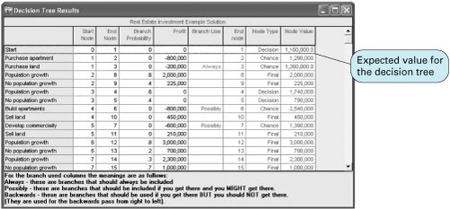 Notice that the expected value for the decision tree, $1,160,000, is given in the first row of the last column on the solution screen in Exhibit 12.14. Sequential Decision Tree Analysis with Excel and TreePlanThe sequential decision tree example shown in Figure 12.5, developed and solved by using TreePlan, is shown in Exhibit 12.15. Although this TreePlan decision tree is larger than the one we previously developed in Exhibit 12.13, it was accomplished in exactly the same way. Exhibit 12.15.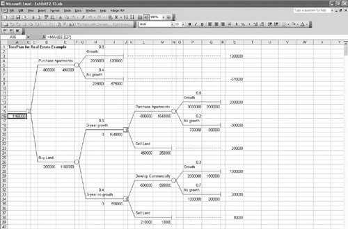 | |||||||||||||||||||||||||||||||||||||||||||||||||||||||||||||||||||||||||||||
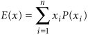
 ) in Figure 12.2 are referred to as
EAN: 2147483647
Pages: 358