Statistical Independence and Dependence
| Statistically, events are either independent or dependent. If the occurrence of one event does not affect the probability of the occurrence of another event, the events are independent . Conversely, if the occurrence of one event affects the probability of the occurrence of another event, the events are dependent . We will first turn our attention to a discussion of independent events. Independent EventsWhen we toss a coin, the two eventsgetting a head and getting a tailare independent. If we get a head on the first toss, this result has absolutely no effect on the probability of getting a head or a tail on the next toss. The probability of getting either a head or a tail will still be .50, regardless of the outcomes of previous tosses. In other words, the two events are independent events . A succession of events that do not affect each other are independent events . When events are independent, it is possible to determine the probability of both events occurring in succession by multiplying the probabilities of each event. For example, what is the probability of getting a head on the first toss and a tail on the second toss? The answer is P (HT) = P (H) P (T) where
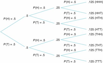
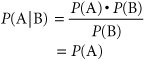
Therefore, P (HT) = P (H) P (T) = (.5)(.5) = .25 The probability of independent events occurring in succession is computed by multiplying the probabilities of each event . As we indicated previously, the probability of both events occurring, P (HT), is referred to as the joint probability . Another property of independent events relates to conditional probabilities . A conditional probability is the probability that event A will occur given that event B has already occurred. This relationship is expressed symbolically as A conditional probability is the probability that an event will occur, given that another event has already occurred . P (AB) The term in parentheses, "A slash B," means "A, given the occurrence of B." Thus, the entire term P (AB) is interpreted as the probability that A will occur, given that B has already occurred. If A and B are independent events, then P (AB) = P (A) In words, this result says that if A and B are independent, then the probability of A, given the occurrence of event B, is simply equal to the probability of A. Because the events are independent of each other, the occurrence of event B will have no effect on the occurrence of A. Therefore, the probability of A is in no way dependent on the occurrence of B. In summary, if events A and B are independent, the following two properties hold: 1. P (AB) = P (A) P (B) 2. P (AB) = P (A) Probability TreesConsider an example in which a coin is tossed three consecutive times. The possible outcomes of this example can be illustrated by using a probability tree , as shown in Figure 11.3. Figure 11.3. Probability tree for coin- tossing example The probability tree in Figure 11.3 demonstrates the probabilities of the various occurrences, given three tosses of a coin. Notice that at each toss, the probability of either event's occurring remains the same: P (H) = P (T) = .5. Thus, the events are independent. Next, the joint probabilities of events occurring in succession are computed by multiplying the probabilities of all the events. For example, the probability of getting a head on the first toss, a tail on the second, and a tail on the third is .125: P (HTT) = P (H) P (T) P (T) = (.5)(.5)(.5) = .125 However, do not confuse the results in the probability tree with conditional probabilities. The probability of a head and then two tails occurring on three consecutive tosses is computed prior to any tosses taking place. If the first two tosses have already occurred, the probability of getting a tail on the third toss is still .5: P (THT) = P (T) = .5 The Binomial DistributionSome additional information can be drawn from the probability tree of our example. For instance, what is the probability of achieving exactly two tails on three tosses? The answer can be found by observing the instances in which two tails occurred. It can be seen that two tails in three tosses occurred three times, each time with a probability of .125. Thus, the probability of getting exactly two tails in three tosses is the sum of these three probabilities, or .375. The use of a probability tree can become very cumbersome, especially if we are considering an example with 20 tosses. However, the example of tossing a coin exhibits certain properties that enable us to define it as a Bernoulli process . The properties of a Bernoulli process follow:
Given the properties of a Bernoulli process, a binomial distribution function can be used to determine the probability of a number of successes in n trials. The binomial distribution is an example of a discrete distribution because the value of the distribution (the number of successes) is discrete, as is the number of trials. The formula for the binomial distribution is where
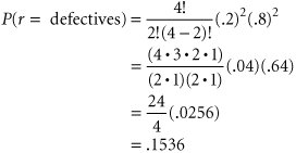
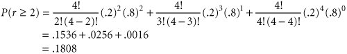
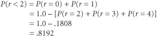
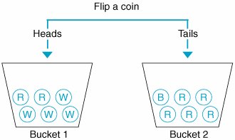
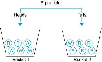
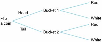
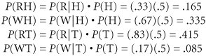
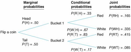
A binomial distribution indicates the probability of r successes in n trials . The terms n !, ( n r)!, and r ! are called factorials . Factorials are computed using the formula m ! = m ( m 1)( m 2)( m 3) . . . (2)(1) The factorial 0! always equals one. The binomial distribution formula may look complicated, but using it is not difficult. For example, suppose we want to determine the probability of getting exactly two tails in three tosses of a coin. For this example, getting a tail is a success because it is the object of the analysis. The probability of a tail, p , equals .5; therefore, q = 1 .5 = .5. The number of tosses, n , is 3, and the number of tails, r , is 2. Substituting these values into the binomial formula will result in the probability of two tails in three coin tosses: Notice that this is the same result achieved by using a probability tree in the previous section. Now let us consider an example of more practical interest. An electrical manufacturer produces microchips. The microchips are inspected at the end of the production process at a quality control station. Out of every batch of microchips, four are randomly selected and tested for defects. Given that 20% of all transistors are defective, what is the probability that each batch of microchips will contain exactly two defective microchips? The two possible outcomes in this example are a good microchip and a defective microchip. Because defective microchips are the object of our analysis, a defective item is a success. The probability of a success is the probability of a defective microchip, or p = .2. The number of trials, n , equals 4. Now let us substitute these values into the binomial formula: Thus, the probability of getting exactly two defective items out of four microchips is .1536. Now, let us alter this problem to make it even more realistic. The manager has determined that four microchips from every large batch should be tested for quality. If two or more defective microchips are found, the whole batch will be rejected. The manager wants to know the probability of rejecting an entire batch of microchips, if, in fact, the batch has 20% defective items. From our previous use of the binomial distribution, we know that it gives us the probability of an exact number of integer successes. Thus, if we want the probability of two or more defective items, it is necessary to compute the probability of two, three, and four defective items: P ( r Substituting the values p = .2, n = 4, q = .8, and r = 2, 3, and 4 into the binomial distribution results in the probability of two or more defective items: Thus, the probability that a batch of microchips will be rejected due to poor quality is .1808. Notice that the collectively exhaustive set of events for this example is 0, 1, 2, 3, and 4 defective transistors. Because the sum of the probabilities of a collectively exhaustive set of events equals 1.0, P ( r = 0, 1, 2, 3, 4) = P ( r = 0) + P ( r = 1) + P ( r = 2) + P ( r = 3) + P ( r = 4) = 1.0 Recall that the results of the immediately preceding example show that P ( r = 2) + P ( r = 3) + P ( r = 4) = .1808 Given this result, we can compute the probability of "less than two defectives" as follows : Although our examples included very small values for n and r that enabled us to work out the examples by hand, problems containing larger values for n and r can be solved easily by using an electronic calculator. Dependent EventsAs stated earlier, if the occurrence of one event affects the probability of the occurrence of another event, the events are dependent events . The following example illustrates dependent events. Two buckets each contain a number of colored balls. Bucket 1 contains two red balls and four white balls, and bucket 2 contains one blue ball and five red balls. A coin is tossed. If a head results, a ball is drawn out of bucket 1. If a tail results, a ball is drawn from bucket 2. These events are illustrated in Figure 11.4. Figure 11.4. Dependent events In this example the probability of drawing a blue ball is clearly dependent on whether a head or a tail occurs on the coin toss. If a tail occurs, there is a 1/6 chance of drawing a blue ball from bucket 2. However, if a head results, there is no possibility of drawing a blue ball from bucket 1. In other words, the probability of the event "drawing a blue ball" is dependent on the event "flipping a coin." Like statistically independent events, dependent events exhibit certain defining properties. In order to describe these properties, we will alter our previous example slightly, so that bucket 2 contains one white ball and five red balls. Our new example is shown in Figure 11.5. The outcomes that can result from the events illustrated in Figure 11.5 are shown in Figure 11.6. When the coin is flipped , one of two outcomes is possible, a head or a tail. The probability of getting a head is .50, and the probability of getting a tail is .50: P (H) = .50 P (T) = .50 Figure 11.5. Another set of dependent events Figure 11.6. Probability tree for dependent events As indicated previously, these probabilities are referred to as marginal probabilities. They are also unconditional probabilities because they are the probabilities of the occurrence of a single event and are not conditional on the occurrence of any other event(s). They are the same as the probabilities of independent events defined earlier, and like those of independent events, the marginal probabilities of a collectively exhaustive set of events sum to one . Once the coin has been tossed and a head or tail has resulted, a ball is drawn from one of the buckets. If a head results, a ball is drawn from bucket 1; there is a 2/6, or .33, probability of drawing a red ball and a 4/6, or .67, probability of drawing a white ball. If a tail resulted, a ball is drawn from bucket 2; there is a 5/6, or .83, probability of drawing a red ball and a 1/6, or .17, probability of drawing a white ball. These probabilities of drawing red or white balls are called conditional probabilities because they are conditional on the outcome of the event of tossing a coin. Symbolically, these conditional probabilities are expressed as follows: The first term, which can be expressed verbally as "the probability of drawing a red ball, given that a head results from the coin toss," equals 33. The other conditional probabilities are expressed similarly. Conditional probabilities can also be defined by the following mathematical relationship. Given two dependent events A and B, the term P (AB) is the joint probability of the two events, as noted previously. This relationship can be manipulated by multiplying both sides by P (B), to yield P (AB) P (B) = P (AB) Thus, the joint probability can be determined by multiplying the conditional probability of A by the marginal probability of B. Recall from our previous discussion of independent events that P (AB) = P (A) P (B) Substituting this result into the relationship for a conditional probability yields which is consistent with the property for independent events. Returning to our example, the joint events are the occurrence of a head and a red ball, a head and a white ball, a tail and a red ball, and a tail and a white ball. The probabilities of these joint events are as follows: The marginal, conditional, and joint probabilities for this example are summarized in Figure 11.7. Table 11.1 is a joint probability table , which summarizes the joint probabilities for the example. Figure 11.7. Probability tree with marginal, conditional, and joint probabilities Table 11.1. Joint Probability Table
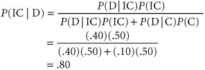
Bayesian AnalysisThe concept of conditional probability given statistical dependence forms the necessary foundation for an area of probability known as Bayesian analysis . The technique is named after Thomas Bayes, an eighteenth-century clergyman who pioneered this area of analysis. In Bayesian analysis, additional information is used to alter the marginal probability of the occurrence of an event . The basic principle of Bayesian analysis is that additional information (if available) can sometimes enable one to alter (improve) the marginal probabilities of the occurrence of an event. The altered probabilities are referred to as revised , or posterior , probabilities. A posterior probability is the altered marginal probability of an event, based on additional information . The concept of posterior probabilities will be illustrated using an example. A production manager for a manufacturing firm is supervising the machine setup for the production of a product. The machine operator sets up the machine. If the machine is set up correctly, there is a 10% chance that an item produced on the machine will be defective; if the machine is set up incorrectly, there is a 40% chance that an item will be defective. The production manager knows from past experience that there is a .50 probability that a machine will be set up correctly or incorrectly by an operator. In order to reduce the chance that an item produced on the machine will be defective, the manager has decided that the operator should produce a sample item. The manager wants to know the probability that the machine has been set up incorrectly if the sample item turns out to be defective. The probabilities given in this problem statement can be summarized as follows: where
The posterior probability for our example is the conditional probability that the machine has been set up incorrectly, given that the sample item proves to be defective, or P (ICD). In Bayesian analysis, once we are given the initial marginal and conditional probabilities, we can compute the posterior probability by using Bayes's rule , as follows: Previously, the manager knew that there was a 50% chance that the machine was set up incorrectly. Now, after producing and testing a sample item, the manager knows that if it is defective, there is an .80 probability that the machine was set up incorrectly. Thus, by gathering some additional information, the manager can revise the estimate of the probability that the machine was set up correctly. This will obviously improve decision making by allowing the manager to make a more informed decision about whether to have the machine set up again. In general, given two events, A and B, and a third event, C, that is conditionally dependent on A and B, Bayes's rule can be written as | ||||||||||||||||||||||||||||||||||||||||||||||||||

 2) =
2) = 

EAN: 2147483647
Pages: 358