Nonlinear Model Examples
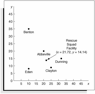
| In our previous profit analysis examples, the models followed the traditional mathematical (i.e., linear) programming formulation, with an objective function, decision variables , and constraints. However, many types of problems employ well-known nonlinear functions but are not typically thought of in the traditional math programming model framework. In this section we consider several additional examples that include familiar nonlinear functionsthe facility location model and the investment portfolio selection model. Facility LocationIn the facility location problem, the objective, in general, is to locate a centralized facility that serves several customers or other facilities to minimize distance or miles traveled between the facility and its customers. This problem uses as a measure of distance the formula for the straight-line distance between two points on a set of x, y coordinates, which is also the hypotenuse of a right triangle: where ( x, y ) = coordinates of proposed facility ( x i , y i ) = coordinates of customer or location facility, i Consider, for example, the Clayton County Rescue Squad and Ambulance Service, which serves five rural towns, Abbeville, Benton, Clayton, Dunning, and Eden. The rescue squad wants to construct a centralized facility and garage to minimize its total annual travel mileage to the towns. The locations of the five towns in terms of their graphical x, y coordinates, measured in miles relative to the point x = 0, y = 0, and the expected number of annual trips the squad will have to make to each town are as follows :
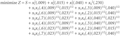
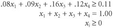
The objective of the problem is to determine a set of coordinates ( x, y ) for the rescue squad facility that minimizes the total miles traveled to the town, according to the following function: where d i = distance to town i t i = annual trips to town i The Excel solution to this problem is shown in Exhibit 10.12. The coordinates ( x, y ) for the new rescue squad facility are in cells C14:C15 . The formulas for the distances between the rescue squad facility and each of the towns ( d i ) are in cells E6:E10 . For example, the formula for the distance, d A , between the rescue squad facility and Abbeville in cell E6 is =SQRT (( B6C14 )^ 2 +( C6C15 )^ 2 ). The formula for the total annual distance in cell D18 is =SUMPRODUCT ( E6:E10,D6:D10 ), which is also shown on the formula bar at the top of the spreadsheet. In the Solver window for this problem, D18 is the target cell that is minimized, and the changing cells (i.e., decision variables) are C14:C15 . There are no constraints. Exhibit 10.12.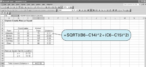 The location of the rescue squad facility is shown graphically in Figure 10.8. Figure 10.8. Rescue squad facility location Investment Portfolio SelectionA classic example of nonlinear programming is the investment portfolio selection model developed by Harry Markowitz in 1959. This model is based on the assumption that most investors are concerned with two factorsreturn on investment and risk. Thus, the objective of the portfolio selection model is to minimize some measure of portfolio risk while achieving a minimum return on the total portfolio investment. Risk is reflected by the variability in the value of the investment, and in this model, variance in the return on investment is the measure of risk. Covariance, which is a measure of correlation, is also used to reflect risk. Individual investment returns within a portfolio typically exhibit statistical dependence. Over time, the returns of any two stocks may exhibit positive or negative correlation; that is, two stocks of the same general type will go up or down together. To adjust for this possible correlation, investors often attempt to diversify their portfolios. To reflect the risk associated with not diversifying, the model includes covariance. The minimization of portfolio risk, as measured by the portfolio variance, is the model objective. The variance, S , on the annual return from the portfolio, is determined by the following formula: where x i , x j = the proportion of money invested in investments i and j r ij = the correlation between returns on investments i and j s i , s j = the standard deviations of returns for investments i and j In the preceding formula for S , the first part is a measure of variance, and the second part is a measure of the covariance. In many cases, the parameters in this equation may be estimates or sample values (the sample variance, sample covariance, etc.). The general formulation of the portfolio selection model is as follows. The investor desires to achieve a minimum expected annual return from the portfolio, which is formulated as a model constraint as follows: r i x i + r 2 x 2 + . . . + r n x n where r i = expected annual return on investment i x i = proportion (or fraction) of money invested in investment i r m = minimum desired annual return from the portfolio A second constraint specifies that all the money is invested: x 1 + x 2 + . . . + x n = 1.0 The following example and Excel solution will demonstrate how this model is applied. Jessica Todd has identified four stocks she wants to include in her investment portfolio. She wants a total annual return of at least .11. From historical data, she has estimated the average returns and variances for the four investments as follows:
She has also estimated the covariances between the stocks, as follows:
The nonlinear programming model formulation for this problem is as follows: subject to The Excel spreadsheet for Jessica Todd's portfolio is shown in Exhibit 10.13. The decision variables representing the proportion of each stock in the portfolio ( x i ) are in cells E6:E9 . The formula for total return, =SUMPRODUCT ( B6:B9, E6:E9 ), is in cell B19. The objective is to minimize the total portfolio variance formula, which is shown on the formula bar at the top of the spreadsheet. This is a complicated formula and difficult to type in. Notice that it has been shortened slightly by doubling the covariance terms in the last part of the equation to reflect all the different investment pairs that are included in B14:E17 (i.e., 2 times AB, AC, AD, BC, BD, and CD will include BA, CA, DA, CB, DB, and DC). In other words, all the covariance terms to the right of the diagonal in the matrix B14:E17 are doubled to include the same values to the left of the diagonal. Exhibit 10.13.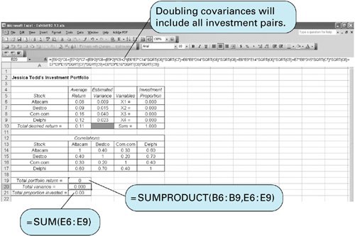 The Solver Parameters window is shown in Exhibit 10.14. Notice that nonnegativity constraints for the variables are included E6:E9 Exhibit 10.14.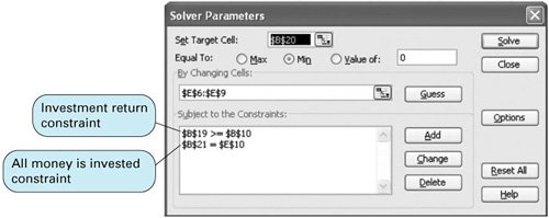 Exhibit 10.15.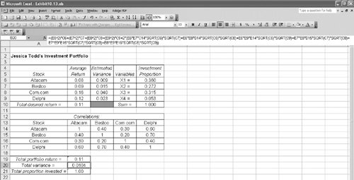 | ||||||||||||||||||||||||||||||||||||||||||||||||||||||||||

EAN: 2147483647
Pages: 358