11.3 Arbitrage-free framework

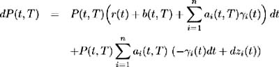
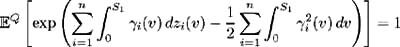
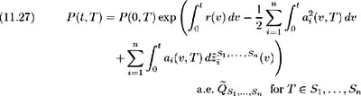
In (11.13) we found the bond price process, under the probability measure Q , to be:

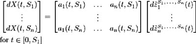
Absence of arbitrage may be equated to the existence of a probability measure such that all discounted security prices are martingales [ 22 ]. We wish to find this martingale probability measure such that it is equivalent ^[9] to the market measure Q and the drift in (11.13) becomes r ( t ). Hence we wish to find a vector of Brownian motions { ( t ), , ( t ): t ˆˆ [0, ]} with n 1 (and associated adapted processes { ³ _i ( t ); t ˆˆ [0, ]} which define ( t ) = ˆ’ ˆ« ^t ³ _i ( u ) du + z _i ( t ), i = 1, , n ) such that ^[10] :

with

Since, by definition, b ( t, T ) represents the cumulative drift of forward rates over [ t, T ], (11.17) implies a restriction is required on the forward rate process to ensure arbitrage-free pricing.

11.3.1 Specification of the martingale measure.

Let us examine necessary and sufficient conditions on the forward rate process ensuring the existence of a unique, equivalent martingale measure and hence arbitrage-free pricing.

Condition 4

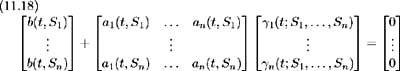
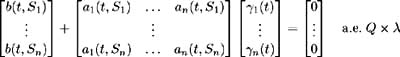
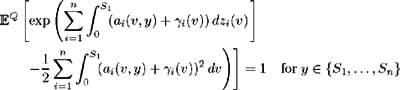
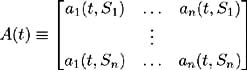
Existence of the market prices of risk. Set S ₁ , , S _n ˆˆ [0, ] such that 0 < S ₁ < S ₂ < < S _n and let » be a Lebesque measure. Assume there exist solutions

to a system of equations specified as:

Also assume that these solutions satisfy the following three conditions ^[11] :

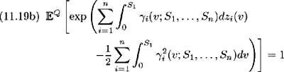
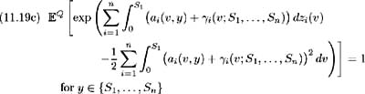
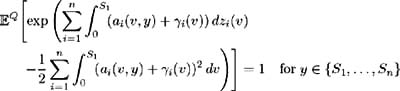
for y ˆˆ { S ₁ , , S _n }

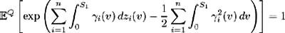
From the system of equations (11.18), we may view ³ _i ( t ; S ₁ , , S _n ), i = 1, , n , as the market prices of risk associated with each source of uncertainty, that is with each Brownian motion z _i ( t ), i = 1, , n .

The market price of risk is defined as the mean rate of return in excess of the risk-free rate of interest, normalised by the volatility of that return. From (11.13) the instantaneous expected return on a T -maturity bond is r ( t ) + b ( t, T ) with a _i ( t, T ), i = 1, , n , the corresponding instantaneous standard deviations of bond return due to the i ^th random factor. Therefore, interpreting ³ _i ( t ; S ₁ , , S _n ), i = 1, , n , as the market prices of risk associated with the sources of uncertainty, this market price of risk relationship may be expressed as:

where the market prices of risk ³ _i ( t ; S ₁ , , S _n ), i = 1, , n , depend on the specific choice of bond maturities { S ₁ , , S _n }. We see that (11.20) is equivalent to (11.17) which was derived using a heuristic argument ^[12] .

The above Condition 4 guarantees the existence of an equivalent martingale measure. This is shown by means of the following proposition.

Proposition 1

Existence of an equivalent martingale probability measure. Set S ₁ , , S _n ˆˆ [0, ] such that 0 < S ₁ < S ₂ < < S _n . Given a vector of forward rate drifts { ± (·, S ₁ ), , ± (·, S _n )} and volatilities { ƒ _i (·, S ₁ ), , ƒ _i (·, S _n )}, i = 1, , n , which satisfy Conditions 1 - 3, then Condition 4 holds if and only if there exists an equivalent probability measure such that { Z ( t, S ₁ ), , Z ( t, S _n )} are martingales with respect to { F _t : t ˆˆ [0, S ₁ ]}.

Proof

The proof of this proposition is by the following two lemmas.

Lemma 1.1

Assume Conditions 1-3 hold for some fixed { S ₁ , , S _n } ˆˆ [0, ]; 0 < S ₁ < S ₂ < < S _n .

Define

Then ³ _i : [0, ] ’ R for i 1, , n , satisfies the following four conditions:

ˆ« ^{S ₁} ³ _i ² ( v ) dv < + ˆ a.e. Q for i = 1, , n

if and only if there exists a probability measure such that the following are true:

( t ) = z _i ( t ) ˆ’ ˆ« ^t ³ _i ( v ) dv are Brownian motions on {( , F , ), ( F _t ; t ˆˆ [0, S ₁ ])} for i = 1, , n
Z ( t,S _i ) are martingales on {( , F , ), ( F _t ; t ˆˆ [0, S ₁ ])} for i = 1, , n

Proof

In the first part of this proof assume (i)-(iv) hold and show that (a)-(d) hold. Make use of the Girsanov Theorem; see [ 21 , Corollary 13.25]. Properties (ii) and (iii) satisfy the conditions for the Girsanov Theorem, so there exists a probability measure on ( , F ) defined by (a) and a corresponding n -dimensional Brownian motion on ( , F , ) defined by (b).

Consider the stochastic differential equation (11.14) describing the evolution of the relative bond price Z ( t, y ):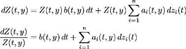

hence

by the definition of X ( t, y ) and for all t ˆˆ [0, y ], y ˆˆ { S ₁ , , S _n }. Therefore:

and from (i) we have:

so: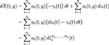

by definition of in (b) and for all t ˆˆ [0, S ₁ ], y ˆˆ { S ₁ , , S _n }. Hence (c) follows .

From (11.21) and (c) we have: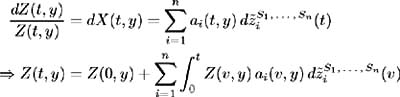

Now by [ 43 , Corollary 3.2.6] Z ( t, y ) is a martingale and hence (d) is satisfied.

Conversely, assume (a)-(d) hold and show that (i)-(iv) are true.

Again by (11.21) and (c) we have:

where ( t ), i =1, , n , a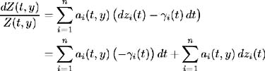re defined in (b) as:

Hence:

But in (11.14) the process for Z ( t, y ) is defined as:

Hence:

and (i) holds. The stochastic integral of any variable ³ _i ( t ) with respect to a Brownian motion z _i ( t ) is defined only if ³ _i ( t ) is square integrable (see [ 30 , Definition 1.5]). Since this integral is defined in (a), ³ _i ( t ) is square integrable, and hence (ii) holds. The Radon-Nikodym derivative (a) defines the relationship between measure Q and 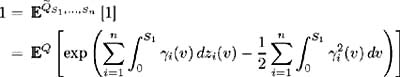; hence:

which proves (iii). We have

and by (d) Z ( t, y ), t ˆˆ [0, S ₁ ], y ˆˆ { S ₁ , S _n } is a martingale, so: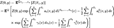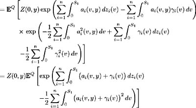

Hence (iv) holds.

Lemma 1.2

Assume Conditions 1-3 hold for some fixed { S ₁ , , S _n [0, ]; 0 < S ₁ < S ₂ < < S _n .

Define

Then there exists a probability measure Q equivalent to Q such that Z ( t, S _i ) are martingales on {( , F , Q ), ( F _t ; t ˆˆ [0, S ₁ ])} for all i = 1, , n , if and only if there exists ³ _i : [0, ] ’ R for i = 1, , n , and a probability measure such that (a), (b), (c) and (d) of Lemma 1.1 hold.

Proof

First, suppose:

there exists a probability measure Q equivalent to Q ,
Z ( t, y ), y ˆˆ { S ₁ , , S _n } are martingales under Q ,

and we need to prove there exists:

³ _i , i = 1, , n ,
probability measure ,

such that (a)-(d) hold.

Since probability measure Q is equivalent to Q we know, by the Radon- Nikodym Theorem (see [ 49 ]), that there exists a non-negative random process N ( t ), t ˆˆ [0, S ₁ ] such that:

For any generic process to be a Radon-Nikodym derivative it must satisfy the following three conditions [ 45 ]:

N (0) = 1,
N ( t ) > 0 for all t ˆˆ [0, S ₁ ],
[ N ( S ₁ ) F _t ] = N ( t ).

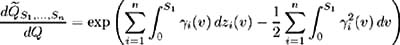
Defining N ( t ) such that:

then (1) and (2) are met. Taking the natural logarithm of N ( t ) we have: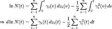

By Ito's Lemma we have: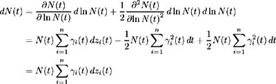

which, by the converse of the martingale representation theorem (see [ 43 ]), implies that N ( t ) is a martingale and (3) holds. All the conditions for N ( t ) to be a valid Radon-Nikodym derivative are met. Hence let be the equivalent probability measure defined by this specific formulation of N ( t ). Then (a) holds, and by the Girsanov Theorem (see [ 43 , Theorem 8.6.4]) the new Brownian motion, ( t ), i = 1, , n , corresponding to the measure is defined by:

and (b) holds.

Z ( t, y ), y ˆˆ { S ₁ , , S _n } are martingales under probability measure Q , more specifically they are martingales under the specific probability measure , and (d) holds. By the martingale representation theorem we may write:

Now we may define 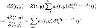i = 1, , n , and so:

However, by the definition of X ( t, y ) we showed above in (11.21) that:

and hence (c) holds.

Conversely, suppose there exist

³ _i , i = 1, , n ,
probability measure ,

such that (a)-(d) are satisfied; we need to prove:

there exists some probability measure Q equivalent to Q ,
Z ( t, S _i ), i = 1, , n , are martingales under Q .

Since and Q are related by the Radon-Nikodym derivative specified in (a) they are equivalent, and we may set Q = . By(d) Z ( t, S _i ), i = 1, , n , are martingales under and since Q = they are martingales under Q .

Hence, by the proofs of Lemma 1.1 and Lemma 1.2 we have proved Proposition 1.

This proposition states that, if Conditions 1-3 are satisfied, then Condition 4 is necessary and sufficient to allow an equivalent martingale measure to exist. An important feature of the proof of this proposition is Girsanov's Theorem, which defines the equivalent martingale measure as:

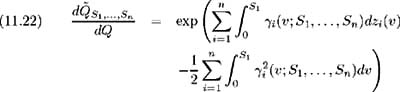
and a new set of independent Brownian motions

on {( , F , ), { F _t : t ˆˆ [0, S ₁ ]}}.

An additional constraint needs to be imposed to guarantee the uniqueness of the equivalent martingale measure.

Condition 5

Uniqueness of the equivalent martingale probability measure. Set S ₁ , , S _n ˆˆ [0, ] such that 0 < S ₁ < S ₂ < < S _n and assume

is non-singular a.e. Q » .

This Condition 5 is both necessary and sufficient to ensure that the equivalent martingale measure is unique. This is proved in the following proposition.

Proposition 2

Uniqueness of the equivalent martingale probability measure. Set S ₁ , , S _n ˆˆ [0, ] such that 0 < S ₁ < S ₂ < < S _n . Given a vector of forward rate drifts { ± (·, S ₁ ), , ± (·, S _n )} and volatilities { ƒ _i (·, S ₁ ), , ƒ _i (·, S _n )}, i = 1, , n , which satisfy Conditions 1-4 then Condition 5 holds if and only if the martingale measure is unique.

Proof

The proof of this proposition is by the following two lemmas.

Lemma 2.1

Set S < and define ² _i : [0, ] ’ R for i = 1, , n , to be such that ˆ« ^S ( v ) dv < + ˆ a.e. Q . Also define:

Then

if and only if { M ^m ( S )} ^ˆ _{m =1} are uniformly integrable.

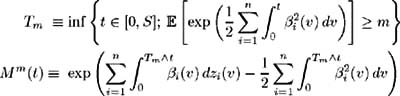
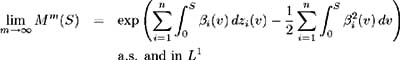
Proof

Since ² _i ( t ), i = 1, , n , is by definition, a square integrable variable on( , F,Q ), then the Ito integral, given by X ^m ( t ) = ˆ‘ _{i =1} ⁿ ˆ« ^{t ˆ§ T _m} ² _i ( v ) dz _i ( v ) follows a continuous martingale on ( , F,Q )[ 41 , Proposition B.1.2.]. Every martingale is a local martingale ^[13] , so by [ 21 , Lemma 13.17]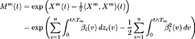

is a supermartingale.

By definition, T _m is the lowest t ˆˆ [0, S ] such that

Hence for all t T _m we have [exp(½ ˆ‘ _{i =1} ⁿ ˆ« ^t ² _i ² ( v ) dv )] m , and in particular [exp (½ ˆ‘ _{i =1} ⁿ ˆ« ^{T _m} ² _i ² ( v ) dv )] m . Hence

and so by [ 21 , Theorem 13.27] the supermartingale M ^m ( t ), t ˆˆ [0, S ] is a martingale and

Now we need to prove both sides of the ˜if and only if' statement:

Assume { M ^m ( S )} ^ˆ _{m =1} are uniformly integrable. By [ 21 , Corollary

Taking expectations:

by (11.24) above.
Conversely, assume

then this is a martingale and so

Hence by [ 21 , Theorem 3.20] { M ^m ( S )} ^ˆ _{m =1} are uniformly integrable.

Lemma 2.2

Assume that Conditions 1-3 hold for a fixed set { S ₁ , , S _n } ˆˆ [0, ], 0 < S ₁ < < S _n . Also assume that the following four conditions of Lemma 1.1 hold:

ˆ« ^{S ₁} ³ _i ² ( v ) dv < + ˆ a.e. Q for i = 1, , n

Then ³ _i ( t ) for i = 1, , n , satisfying the above conditions are unique (up to » Q equivalence) if and only if

is singular with ( » Q ) measure zero.

Proof

First, assume A ( t ) is singular with ( » Q ) measure zero. Since condition (i) holds we have: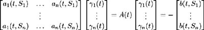

Singularity with measure zero implies A ( t ) is invertible; hence we may solve for unique (up to » Q ) ³ _i ( t )s ; i = 1, , n ,as: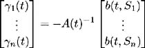

Conversely, define & pound ; as the set on which A ( t ) is singular, that is { t ˆˆ [0, S ] : A ( t ) is singular}. Assume that has ( » Q )( ) > 0. Then proof is by contradiction. Hence, having assumed A ( t ) is singular, we wish to show that the functions satisfying (i)-(iv) are not unique.

Firstly, since (i)-(iv) are assumed to hold, we have a vector of functions ( ³ ₁ ( t ), , ³ _n ( t )) satisfying these conditions.

Part 1 We wish to show that there exists a bounded, adapted and measurable vector of functions ( ₁ ( t ), , _n ( t )) which is non-zero on and satisfies: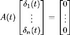

and where g ( t ), defined as:

is bounded a.e. on Q .

Let _i = {( t , ): A ( t ) has rank i }. _i has the following properties:

_i is a measurable set,
= ‹ƒ _{i =1} ^{n ˆ’ 1} _i ,
_i ˆ _j = ˆ for i j ,

Fix ² > 0. On each _i set ^² _i ( t ), i = 1, , n , to be a solution to ^[14] :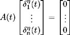

such that ^² _i ( t ) is bounded by min { ² , 1/ ³ _i ( t ) i = 1, , n }. Also, let ^² _i ( t ) be zero on ^c ; i = 1, , n . By construction, ^² _i ( t ) are adapted, measurable and bounded by ² . Also: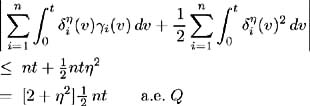

Set ± = inf { j ˆˆ {1, 2, 3, } :(½) ^{2 j} S < 1} and define inductively the following stopping times: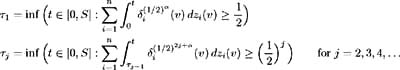

We need to show that the claim Q (lim _{j ’ˆ} _j = S ) = 1 is true. First consider: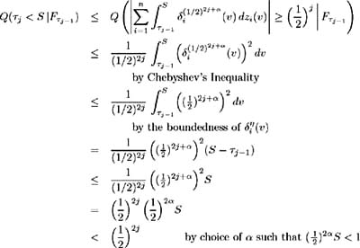

and hence [ Q ( _j < S F _{_{j ˆ’ 1}} ) = Q ( _j < S ) < (½) ^{2 j} . Now consider ^[15] :

Hence:

and we have proved the claim. Set

By this construction of _i ( t ) we know it is bounded, adapted, measurable and satisfies: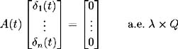

Also for all t ˆˆ [0, S ] we have: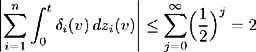

and so

is bounded a.e. » Q . Part 1 is complete.

Part 2 Now to complete the proof, we wish to show that ( ³ ₁ ( t )+ ₁ ( t ), , ³ _n ( t ) + _n ( t )) satisfies (i)-(iv).

Consider condition (i). We need to show that: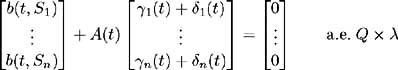

Since ( ³ ₁ ( t ), , ³ _n ( t ) satisfies (i) we have: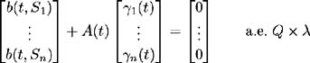

and by construction above

Hence condition (i) is satisfied.

To satisfy condition (ii) we require

Expanding the integration, we have:

Since ³ _i ( v ) satisfies condition (ii) and from Part 1 we know

is bounded, we conclude ( ³ _i ( t ) + _i ( t )), i = 1, , n , satisfy condition (ii).

Condition (iii) requires:

To show that this condition holds, follow the proof of Lemma 2.1. Define: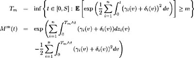

and we need to show that { M ^m ( S )} ^ˆ _{m =1} is uniformly integrable.

We have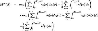

From Part 1 we know that

is bounded by some value, say K > 0. Hence:

and since ³ _i ( t ) satisfies condition (iii), the right-hand side is uniformly integrable and hence it may be shown that M ^m ( S ) is uniformly integrable.

Finally to show that condition (iv) is satisfied, we must show: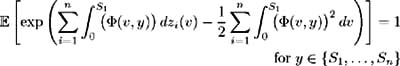

where ( v, y ) = a _i ( v, y ) + ³ _i ( v ) + _i ( v ). Again, following the proof of Lemma 2.1 we define: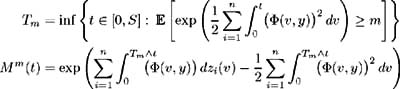

and the condition holds if { M ^m ( S )} ^ˆ _{m =1} is uniformly integrable. M ^m ( S ) may be decomposed as: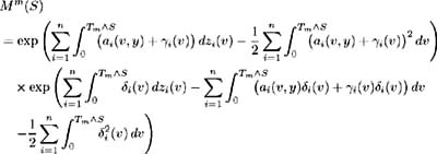

By choice of _i ( v ) in Part 1 we have

and

is bounded by some value, say K > 0. Therefore we may write: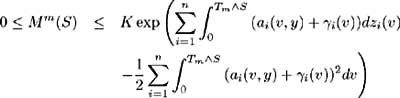

and since ³ _i ( t ) satisfies condition (iv), the right-hand side is uniformly integrable and hence it may be shown that M ^m ( S ) is uniformly integrable.

Hence, by the proofs of Lemma 2.1 and Lemma 2.2 we have proved Proposition 2.

Conditions 1-5 impose restrictions on the market prices of risk, ³ _i ( t ; S ₁ , S _n ), i = 1, , n , which results in restrictions on the drifts of the forward rate processes { ± (·, S ₁ ), , ± (·, S _n )}. These restrictions are required to guarantee the existence of the unique equivalent martingale probability measure for relative bond prices { Z ( t, S ₁ ), , Z ( t, S _n )}, 0 < S ₁ < S ₂ < < S _n .

11.3.2 Model dynamics under the martingale measure.

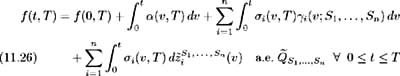
Let us now determine the dynamics of the forward rate and bond price under this equivalent martingale probability measure. In (11.23) the Brownian motions with respect to the equivalent martingale measure are defined as:

Substituting into (11.4), the dynamics of f ( t, T ) under the equivalent martingale measure are:

To determine the bond price process under the equivalent martingale measure, substitute (11.25) into (11.13) and make use of the market price of risk equation (11.20) to give:

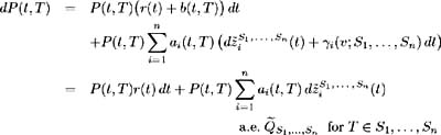
Also from (11.12), the logarithm bond price process, we have:

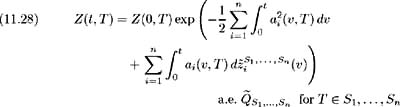
Similarly, the relative bond price under the equivalent martingale measure may be determined from (11.16) as:

Although these processes evolve in a risk-neutral economy, the forward rate process (11.26) (and since r ( t ) = f ( t, t ), also the short- term interest rate process) displays explicit dependence on the market prices of risk, ³ _i ( v ; S ₁ , , S _n ), i = 1, , n . Hence, to price any security depending on either the short or forward interest rate, the market prices of risk must be known.

^[9] Equivalence of two probability measures, Q and implies Q ( A ) = 0 if and only if ( A ) =0, A ˆˆ F , that is, the probability measures have the same null sets [ 24 ].

^[10] This is equivalent to finding an equivalent probability measure such that the relative bond price process (11.14) has no drift term, i.e. may be expressed as:

^[11] [·] is the expectation taken with respect to some probability measure P .

^[12] The two formulae are equivalent up to the former's dependence on a specific choice of bond maturities. However, later in the analysis this dependence is eliminated.

^[13] A local martingale may be defined [ 41 , p. 462] or [ 30 , Definition 1.7] as follows: a stochastic process X =( X ( t )) _t is said to be a local martingale on ( , F,Q ) if there exists an increasing sequence _n of stopping times such that _n tends to T a.s., and for every n the process X ⁿ ( t ), given by the formula X ⁿ ( t ) = X ( t ˆ§ _n ), is a martingale.

^[14] Here we iteratively build vector ^² ( t ). That is for each _i we determine element ^² _i ( t ), until the entire vector has been determined.

^[15] This result is by Fatou's Lemma, e.g. see [ 41 ].