10.4 Relationship to Vasicek and CIR models

The Vasicek [ 50 ] and CIR [ 18 ] models describe the instantaneous short-term interest rate by means of a stochastic process. Within the discrete time HL model, the short- term interest rate equivalent is the one period rate. To make a meaningful comparison of these models we need to find the stochastic process described by the evolution of this rate in the binomial lattice.

10.4.1 Calculating the continuous time equivalent.

10.4.1.1 General functional form.

Rebonato [ 45 ] presents a simple analysis by which the continuous time equivalent of a discrete time model, modelled within a binomial lattice, may be found.

At each time step t in a binomial lattice, there are t + 1 possible states of the world and hence t + 1 possible values of the one period rate. Consider time t = 1, there are two possible states of the world and interest rates, denoted r (1, 1) and r (1, ˆ’ 1). Given the assumption that the short-term interest rate follows a Gaussian process, the standard deviation of the time t = 1 one-period rate may be represented as:

where ƒ is the absolute volatility of the one period rate.

Let r _m (1) be the median interest rate at time t = 1; hence:

and

and so, in continuous time, we may write:

where u ( t ) is time t median of the short-term interest rate distribution, ƒ is the constant short-term interest rate volatility and z ( t ) is a standard Brownian motion. Now, apply Ito's Lemma to determine the stochastic process for the short-term interest rate, r ( t )= r ( t, z ( t )):

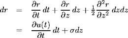
Letting , the process for the short-term interest rate may be expressed as:

where ( t ) is a function of the initial term structure. This is the case since u ( t ), the median of the short-term interest rate, is determined as part of the binomial tree calibration process.

10.4.1.2 Specific functional form of ( t ) dependent on lattice parameters.

Now we examine how this drift function, ( t ), is dependent on the specific parameters of the binomial tree. First, we make use of (10.5) and (10.6) to determine the discount function at time n , state i , in terms of the initial discount function and the perturbations required to get there. Equations (10.5) and (10.6) are:

Repeated application of (10.27) yields:

and

Hence:

Eventually we arrive at the formula:

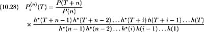
The above combination of perturbation functions results from the i upstate moves and ( n ˆ’ i ) downstate moves required to reach the i ^th state at time n . The order of the moves is not important since the time n , state i , discount function is path -independent. Equation (10.28) can be used without loss of generality.

From (10.22) and (10.23) we have:

Hence (10.28) may be written as:

^[8]

where the exponent of is consistent with requiring ( n ˆ’ i ) downstate moves (and i upstate moves) to reach time n , state i .

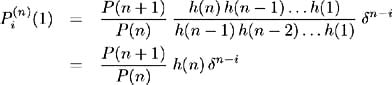
Now, consider the special case of a one-period bond i.e. T =1. From (10.29) we have:

But, from (10.22) we have:

Hence:

To represent the interest rate term structure in terms of yields as opposed to discount functions, let r ( T ) be the continuously compounded yield on a discount bond of maturity T ; then:

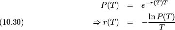
and so the time n , state i , one period yield may be expressed as:

Thevalueof i , that is the possible state at time n , has a Binomial distribution ^[9] with probability q . Hence at time n the mean value of i is ¼ ( i ) = nq . Since r ^{( n )} _i (1) is unique for every state and time, it also has a Binomial distribution in i for each time n . The mean of this distribution, that is the mean short-term interest rate at time n , may be calculated from (10.31) as:

The first term in (10.32) is the implied forward rate, while the other two terms give the bias introduced by uncertainty, i.e. which gives the ratio of the upstate and downstate perturbations. Consider the drift of the short- term interest rate ( t ), in (10.25). This drift is chosen so as to fit the initial observed term structure. This dependence on the initial term structure is represented by the first term in (10.32), i.e. the implied forward rate. The time dependence of ( t ) is indicated by the parameter n , in each of the three terms of (10.32).

The variance of the short-term interest rate may be calculated from (10.31) as follows:

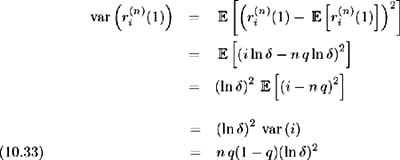
As the spread between the up and down perturbation functions ( h ( ·) and h *( ·)) increases , so the value of decreases ^[10] . An increase in this spread implies an increase in variance, hence the variance is negatively related to .

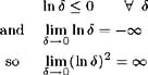
Consider the volatility ƒ , of the short-term interest rate defined in (10.25). This is the instantaneous volatility, hence for a specified time period the volatility is ƒ ˆ t . From (10.33) the corresponding time n short-term interest rate volatility is ln . Therefore the constant value ƒ is represented by ln since and q are constant parameters ^[11] associated with the binomial lattice.

10.4.2 Comparing the modelling techniques.

By calculating the mean and variance of the short-term interest rate, we have specified the stochastic process that governs its evolution. This stochastic process depends on information contained in the initial term structure; therefore the future evolution of the short-term interest rate is determined by the initial term structure. Traditional one factor models, such as the Vasicek and CIR ^[12] models, do not fit the initial term structure exactly since they specify the short-term interest rate process exogenously. These two different approaches (that is the Vasicek/CIR on one hand and HL on the other) may be justified since they are each applied for a different purpose. The traditional one-factor models, such as the Vasicek and CIR models, endogenise the equilibrium term structure by attempting to determine a short-term interest rate process that generates a meaningful equilibrium term structure. The purpose of the approach taken by HL is not to determine an equilibrium term structure, but rather to price contingent claims consistently with respect to the initial term structure. For this reason the short-term interest rate movements incorporate information from the initial term structure.

^[8] Considering the terms in the numerator, we have:

Here the exponent may be written as:

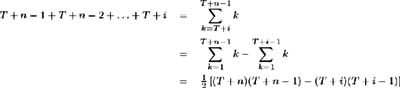
Similarly, the exponent of the terms in the denominator may be expressed as:

Then, to simplify, we subtract the exponent of in the denominator from the exponent of in the numerator to yield:

^[9] At each step of the Binomial tree the movement of the discount function is subject to a Bernoulli trial. A Bernoulli trial has one of two possible outcomes - success (1) or failure (0), where q denotes the probability of success. The Binomial distribution is made up of n identical Bernoulli trials. It has the following characteristics:

^[10] is defined as h *( ·)/ h ( ·) that is, the down perturbation function divided by the up perturbation function, hence ‰ 1 for all values of h ( ·) and h *( ·). As the spread between the two functions increases, so tends to zero. Therefore:

Hence the increasing value of the variance with decreasing value of .

^[11] Parameter q is the binomial probability corresponding to the risk-neutral probability characterising the lattice.

^[12] In the most general form, the process used by the traditional Vasicek and CIR models is:

where , and ƒ are constants. In the Vasicek model ² = 0 while in the CIR model ² = ½. Since none of the parameters are time-dependent, only the initial short-term interest rate can be fitted to a rate observed in the market.