7.5 Fitting model parameters to market data

To use either model for contingent claim pricing, the functions A (0, T ) and B (0, T ) must be estimated. By determining the relationship of A (0, T ) and B (0, T ) to the initial term structure of interest rates and volatilities, historical data may be used to estimate these functions.

7.5.1 Relationship between B (0, T ) and the current term structure of interest rates.

We derive the relationship between B ( t, T ) and the current term structure of interest rates and interest rate volatilities. Here, volatility refers to the standard deviation of proportional, rather than absolute, changes in interest rates.

The time t price of a discount bond with unit maturity value and maturity time T , is simply the unit maturity value discounted to time t using the appropriate rate of interest i.e.

where R ( r, t, T ) represents the continuously compounded time t rate of interest applicable for the period ( t, T ). Since, by equation (7.6) the bond price takes the form:

we have

and so

Applying Ito's Lemma to determine the stochastic process for R ( r, t, T )we have ^[6] :

Hence:

where ƒ _R ( r, t, T ) represents the volatility of R ( r, t, T ). Now, from (7.35) and (7.36) we have:

This equation represents the relationship between B ( t, T ) and

the instantaneous short-term interest rate,
the term structure of spot interest rates,
instantaneous volatility and
the term structure of volatilities.

Therefore given the current term structure of spot interest rate volatilities, (7.37) may be used to determine B (0, T ) for all T .

Alternatively, consider the relationship between spot interest rates and forward rates where F ( r, t, T ₁ , T ₂ ) is the time t forward rate applicable for period ( T ₁ , T ₂ ). We have:

Again, applying Ito's Lemma, allows us to determine the volatility of the forward rate, hence:

and so the standard deviation of F ( r, t, T ₁ , T ₂ )is:

However, F ( r, t, T ₁ , T ₂ ) is a function of R ( r, t, T ₁ ) ‰ R ₁ and R ( r, t, T ₂ ) ‰ R ₂ which in turn , are functions of r , therefore:

and so by (7.35) and (7.38) we have:

Substituting into (7.39) gives:

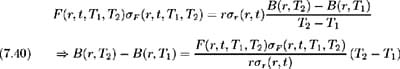
The above equation gives the relationship between B ( t, T ₁ ) and B ( t, T ₂ ) and

the instantaneous short-term interest rate,
instantaneous volatility,
the term structure of forward rates and
the term structure of forward rate volatilities.

Here (7.37) and (7.40) represent two ways by which B (0, T ) may be obtained for all T , either as a function of the current term structure of spot interest rate volatilities or as a function of the current term structure of forward rate volatilities.

7.5.2 Determining A (0, T ) from the current term structure.

Knowing the current interest rate term structure implies that the current prices of zero coupon bonds are known for all maturities, i.e. we know P ( r, 0, T ) for all T . Evaluating equation (7.18) at t = 0 gives ^[7] :

Knowing B (0, T ) we may determine A (0, T ) for all T from the above relationship as

Alternatively, since it is possible to find analytical solutions to European option prices under the Vasicek model, historical interest rate term structure and option price data can be used to imply the values of A (0, T ) and B (0, T ) by means of equations (7.20) and (7.24).

7.5.3 Stability of fitted parameters.

For a model to be a good description of term structure movements through time, the fitted model parameters A ( t, T ) and B ( t, T ) need to remain stable through time. That is, parameters fitted to the term structure of interest rates and interest rate volatilities at time t ₁ need to be the same as the parameters fitted to the term structure of interest rates and interest rate volatilities at time T, t ₁ ‰ T . Hence, a model fitted at one time, should correctly describe the term structure at some other time.

The extended Vasicek model does not meet these criteria and hence appears to be unsuitable for this application. However, the goal here has been to develop a model which correctly values most of the interest rate contingent claims in the market. Initially fitting the model to observed prices of vanilla instruments then allows more exotic instruments to be valued consistently.

^[6] Here the price process of the instantaneous short-term interest rate r is represented as dr = adt + r ƒ _r ( r, t ) dz where ƒ _r ( r, t ) is the volatility of r (i.e. standard deviation of relative changes).

^[7] The explicit functional dependence of r on current time t has, until now, been suppressed to streamline the notation. Here r (0) explicitly denotes the time t = 0 short-term interest rate.