2.7 Distribution of the interest rate

2.7.1 Mean.

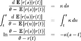
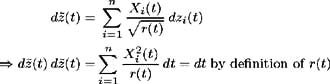
To calculate the conditional mean and variance of the interest rate under the CIR model ^[11] , consider the integral form of (2.17):

since r ( t ), the current rate of interest is known. The mean of a Wiener process is zero, and so taking expectations:

In differential form this equation is represented as:

which is a separable differential equation which may be solved as follows :

2.7.2 Variance.

Calculate the stochastic differential equation satisfied by r ² ( t ) by applying Ito's formula to (2.17). Define f ( x )= x ² then:

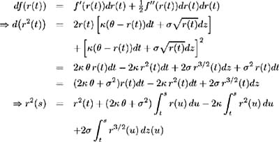
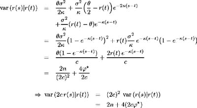
Considering the conditional expectation of r ² ( s ) we have:

Partial differentiation with respect to s yields:

and hence:

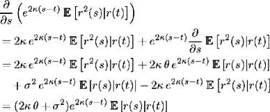
Integrating the above over [ t, s ] and using (2.19) gives:

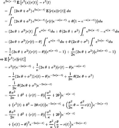
From (2.19) we have:

and so the conditional variance of r ( s )is:

2.7.3 Identifying the distribution.

Define

where each X _i ( t ) is an Ornstein-Uhlenbeck process representing the solution to [ 49 ]:

where ² > 0 and ƒ > 0 are constants and z _i is a Wiener process. The conditional mean of X _i is:

The stochastic process for r ( t ) is derived by application of It 's formula as ^[12] :

By setting = ² and = n ƒ ² /(4 ² ) we arrive at the formulation in (2.17). Defining r ( t ) as the sum of squares of normally distributed ^[13] variables X _i , i = 1, , n leads to the correct form of its stochastic process, hence we may conclude that r ( t ) has a non-central ² distribution.

2.7.4 Chi-Square distribution.

Consider a random variable Y , which may be expressed as:

where the X _i s form a mutually independent set and each X ² _i , i = 1, , d is a standard normal variable, i.e. X _i ˆ¼ (0, 1), i = 1, , d . Y has a ² distribution with d degrees of freedom [ 35 ].

If X _i ˆ¼ ( c _i , 1), i = 1, , d , that is the X _i s are normally distributed with mean c _i and variance 1, then Y has a non-central ² distribution with parameter of non- centrality ˆ ˆ‘ c ² _i and d degrees of freedom [ 35 ]. The mean, variance and probability density function f (·), of Y are expressed as [ 35 ]:

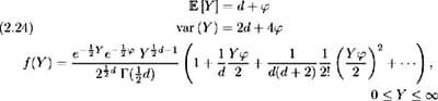
where (·) is the Gamma function ^[14] .

Define the following variables:

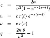
Now calculate the parameters required to characterise the distribution function of r ( s ), conditional on its value at r ( t ). From (2.23) the number of degrees of freedom are:

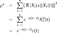
The parameter of non-centrality may be calculated as ˆ * = ˆ‘ c ² _i where c _i , i = 1, , n are the conditional means of the X _i s as specified in (2.22):

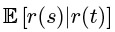
From (2.19) the conditional expectation of the short- term interest rate as specified by the CIR model is:

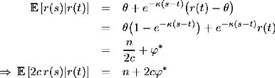
Similarly, the conditional variance of the short-term interest rate is specified by (2.20) as:

So from the definition of the mean and variance of a ² distribution in (2.24) we may conclude that 2 cr ( s ) has a ² distribution with n degrees of freedom and parameter of non-centrality

To determine the probability density function of r ( s ), conditional on its value at time t , use the characterisation of the probability density function of a ² distribution in (2.24) with Y = 2 cr ( s ):

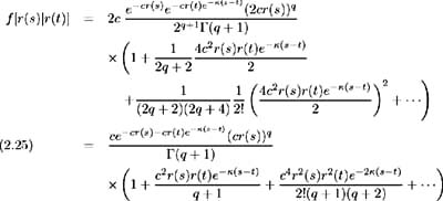
This representation of the conditional probability density function can be shown to be equivalent to the formulation used by CIR in their original paper, which makes use of the modified Bessel function ^[15] :

2.7.5 Mean reversion.

The conditional mean of the short-term interest rate depicted in (2.19) clearly displays its reverting property.

Consider:

if r ( t ) = then r ( s ) = , for all s t ,
if r ( t ) then lim _{s ’ˆ} r ( s ) = ,
for ’ ˆ (where is the reversion speed), ’ , the long-term mean and var ( r ( s ) r ( t )) ’ 0,
for ’ 0, ’ r ( t ), the current rate of interest and var ( r ( s ) r ( t )) ’ r ( t ) ƒ ² ( s ˆ’ t ). ^[16]

In the above cases the properties of the future rate of interest are consistent with our expectations, given the structure of the interest rate dynamics.

If , > 0, i.e. the interest rate is mean reverting, then as s ’ ˆ ,the interest rate approaches the gamma distribution with density function:

where = 2 / ƒ ² and ½ = 2 / ƒ ² . The mean and variance are and ƒ ² /2 respectively which is also consistent with our expectations of the interest rate dynamics ^[17] .

2.7.6 Negative interest rates.

As already identified in §2.7.3 and §2.7.4 r ( t )hasa ² distribution and so it may be written as a sum of squares of normally distributed random variables:

Consider the case: n =1, so r ( t )= X ² ₁ ( t ). Since X ₁ ( t ) is normally distributed, we know that for each t , { r ( t ) 0} = 1. Hence it is also the case that for any t > 0, {There are infinitely many values of t where r ( t )=0} = 1.

Now consider n 2. For r ( t ) = 0, t > 0 we require X _i ( t ) = 0, for every i = 1, , n and so {There exists a t > 0 such that r ( t ) = 0} =0.

Therefore, to prevent zero (and hence negative) interest rates, we require n 2. From the stochastic process describing r ( t ) in (2.23) we have:

The requirement n 2, needed to prevent zero (and hence negative) interest rates translates to:

^[11] See [ 49 ] for detailed calculations of the mean and variance.

^[12] Since r ( t ) = X ² ₁ + X ² ₂ + + X ² _n r ( X ₁ , X ₂ , , X _n ) we have, by the independence of the X _i s:

where the subscripts denote partial derivatives, and so

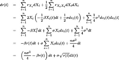
where ( t ) the transformed Brownian motion, is defined as:

To verify that ( t ) is in fact a Brownian motion, consider:

Also, since z _i ( t ), i =1, , n are martingales, then ( t ) is a martingale and we have verified that ( t ) is in fact a valid Brownian motion.

^[13] The X _i s are normally distributed by their specification as Ornstein-Uhlenbeck processes in (2.21).

^[14] The Gamma function is defined as:

and ( ± ) = ( ± ˆ’ 1)! for ± ˆˆ

^[15] I _q (·) is the modified Bessel function of the first kind of order q . This function is defined as:

and so in the CIR probability density function, we have:

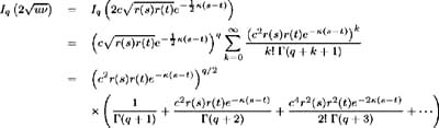
Hence, making use of the identity ( ± + 1) = ± ( ± ), (2.26) expands to:

which is equivalent to the distribution in (2.25).

^[16] Apply L'Hopital's Rule to the first term of (2.20) to obtain

^[17] This mean and variance can also be obtained by letting s ’ ˆ in (2.19) and (2.20).