9.3 Parasitic-aware optimisation
|
9.3 Parasitic-aware optimisation
As intimated above, it becomes virtually impossible to find tractable analytic solutions for RF circuits when all of the parasitic components are considered. Hence, we employ parasitic-aware numerical CAD design and optimisation techniques to find solutions. Conventional gradient descent optimisation techniques are ubiquitous. However, they are not well suited for RF circuit synthesis because they do not possess a probabilistic hill climbing capability, and can therefore easily become trapped in suboptimal local minima in the complex design space. To illustrate this effect, assume the initial design point is in Region I or III (Figure 9.5). Conventional gradient descent methods (Figure 9.6) would find a local minimum at A or C, not the global minimum solution at B. Hence, optimisation methods are required that can find the global minimum for arbitrary initial design points; one such global search heuristic is simulated annealing.
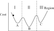
Figure 9.5: Local minima (A and C) and a global minimum (B) for a simple cost function
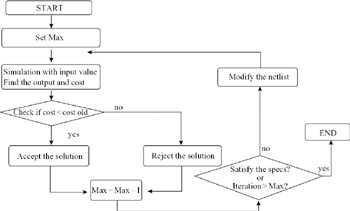
Figure 9.6: Typical flow chart for gradient descent optimisation
9.3.1 Simulated annealing
As the name suggests, the simulated annealing algorithm originated from metal annealing technology. In metal annealing, a product such as a knife is heated to a high temperature during manufacture, and then cooled at an optimum rate so that its total number of defects is minimized. After annealing, the positions of the metal atoms are stable and the bonds between them are strong; in other words, a minimum energy system is created. Simulated annealing mimics this behaviour [4–6].
Simulated annealing provides a statistical hill climbing capability, and thus avoids, with high probability, being trapped in undesired local minima. However, the hill climbing process needs to be controlled to minimise simulation time. In the simulated annealing technique, two controls on the hill climbing process are the slope of the cost function and the Temp coefficient:
![]()
The left side of (9.5) is a random number between 0 and 1, and because of the preceding conditional operation shown in Figure 9.7, oldcost − cost (−Δcost) is always less than 0. Therefore, the right side of (9.5) is also always less than 1. If Temp is high and the right side of (9.5) is close to 1, the probability of hill climbing is high. On the other hand, if Δcost is large, the right side of (9.5) approaches 0, and the probability of hill climbing is low. Table 9.1 summarizes the general relationships between the probability of hill climbing and the coefficients Temp and Δcost.
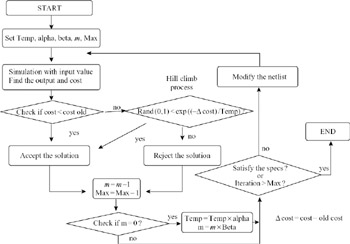
Figure 9.7: Flow chart of the parasitic-aware simulated annealing optimisation methodology
| Probability of hill climb | Temp | Δ(cost) |
|---|---|---|
| | ||
| High | High | Low |
| Low | Low | High |
In an implementation of the simulated annealing algorithm, the parameter Temp is, in turn, controlled by the parameter alpha. Initially, Temp is set to a high value that decreases during optimisation according to the value of alpha. Figure 9.7 shows a typical flow chart of simulated annealing optimisation; it requires the setting of five parameters: alpha, beta, Temp, m and Max. Temp is the temperature parameter required in equation (9.5), and alpha is used in controlling the value of Temp. m is the number of iterations for the same Temp value, and beta is used for controlling the m factor. Max is the maximum number of iterations allowed.
In the gradient descent search optimisation method shown in Figure 9.6, only the slope of the cost function determines if a solution is accepted. In contrast, simulated annealing uses an iterative loop with an optimum temperature-cooling algorithm. Hence, there are more chances of finding an acceptable solution according to equation (9.5).
Figure 9.8 shows the computational flow details of the simulated annealing approach. The simulated annealing code requires a SPICE Netlist, and a setup file that includes the design parameters that are to be optimised, the cost function information, and the parameters described above including Temp, alpha, Max, etc. First, the setup file is used to modify the SPICE Netlist according to the assumed initial solution; then, SPICE is run in order to evaluate the given cost function. After evaluating it, the simulated annealing optimiser conditionally accepts the solution according to the five key parameters. Accepted solutions are saved to the .m file for later analysis and plotting using MATLAB.
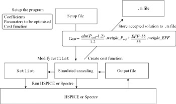
Figure 9.8: Flow diagram of the inner loop of the parasitic-aware simulated annealing algorithm
A parasitic-aware RF CAD design and optimisation tool should exhibit two key features. First, it should find acceptable solutions efficiently in terms of the required number of computer cycles. Second, it should possess the ability to escape local minima in the complex design space in order to maximise the probability of finding the global minimum. While the general simulated annealing algorithm offers a hill climbing capability that usually satisfies the second objective, it has several significant shortcomings for parasitic-aware RF circuit synthesis. A critical parameter in determining the cooling schedule in conventional simulated annealing is the Temp coefficient. Not only is it difficult and time consuming to determine an optimum value for this key empirical parameter, a prohibitive number of iterations is often required to find a suitable set of acceptable solutions once the value of Temp is set.
In this chapter, a simulated annealing algorithm is described that features adaptive determination of the Temp coefficient, and a tunnelling process to speed the global and local searches, respectively. Hence, the computer time required for parasitic-aware RF circuit synthesis is significantly reduced and the probability of finding the global minimum is substantially increased, compared to previous simulated annealing approaches.
9.3.2 Adaptive simulated annealing
The simulated annealing parasitic-aware synthesis approach has three major component parts: the tunnelling process, the local optimisation technique, and the adaptive Temp coefficient method.
9.3.2.1 Tunnelling process
A well-known advantage of simulated annealing is its hill climbing ability, which is determined by the Temp coefficient in the cooling schedule and the slope of the hill. Showing a simple cost function that depends on a single design variable, X, Figure 9.9a depicts hill climbing in conventional simulated annealing. There is a finite non-zero probability of escaping local minima in search of the global minimum. However, if Temp is fixed and the hill is steep, an unacceptably large number of iterations may be required to climb from point A to point B, even though there are no better solutions between those two points as indicated by the higher values of the cost function.
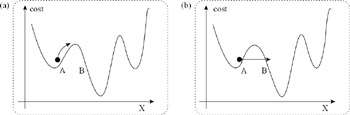
Figure 9.9: (a) Hill climbing in simulated annealing, and (b) the tunnelling process in adaptive simulated annealing for a cost function versus design variable, X
In the case of a genetic optimisation algorithm, this drawback is often overcome using TABU search methods [7]. With TABU, unacceptable points are recorded and not simulated again so the total number of iterations to find an acceptable set of solutions is reduced. However, the TABU method is not reliably applied with the simulated annealing algorithm because it effectively inhibits the hill climbing process. That is, the solution search may become stuck at a local minimum because TABU disallows hill climbing over known unacceptable solutions in search of the optimum.
To achieve the advantages of TABU while avoiding its catastrophic disadvantage in simulated annealing as described above, a new tunnelling technique is developed, as illustrated conceptually in Figure 9.9b. Rather than wasting time hill climbing through aregion of known unacceptable solutions, or getting stuck, theoptimisersimplysenses the beginning of a climb and enables tunnelling from point A to point B. Whereas TABU considers unacceptable solutions only once, the tunnelling method never considers many unacceptable solutions. Hence, the required number of iterations needed in parasitic-aware synthesis is greatly reduced.
Figures 9.10 compares conventional simulated annealing and adaptive simulated annealing with tunnelling. The curves represent a cost function versus values of a single design variable, X. Note that the cost function has several local minima, and that the ‘ ’ and ‘ ’ points portray accepted and unaccepted solutions, respectively. As illustrated in the example of Figure 9.10a, conventional simulated annealing wastes iterations finding unacceptable solutions between points A and B, far above the global minimum (lowest cost) solution. In general, only a small percentage of the solutions are the desired low cost ones.

Figure 9.10: (a) Conventional simulated annealing, and (b) adaptive simulated annealing results for a cost function versus a design variable, x
In contrast, when the tunnelling process is applied as depicted in Figure 9.10b, no acceptable and few unacceptable solutions are considered between points A and B. That is, the searchable design space is reduced because many unacceptable points between A and B are not simulated. Hence, the new tunnelling technique focuses on more desirable lower cost acceptable solutions. Thus, there is a higher probability of finding the global minimum quickly without becoming trapped in a local minimum.
The initial version of the tunnelling algorithm uses two key parameters called the tunnelling threshold and the tunnelling radius. The tunnelling threshold determines the conditions when tunnelling is invoked, while the tunnelling radius specifies the maximum distance a simulation point tunnels in the design space. The tunnelling radius is a critical coefficient in the tunnelling process. If it is too small, the probability of tunnelling through a hill is low; if it is too large, the solution might tunnel so far past the optimum solution that it may never be found. A simple method of determining the tunnelling radius is described below.
Figure 9.11 shows a flow chart of the tunnelling process. As indicated, when tunnelling occurs, a fraction of the tunnelling radius is added to the previous parameter values to determine the new design variable values.
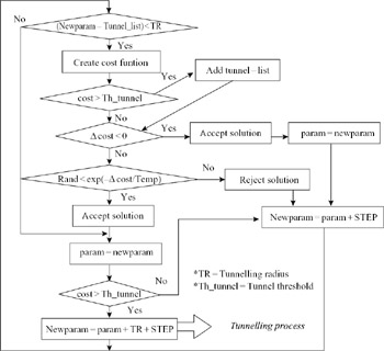
Figure 9.11: Flow chart of simulated annealing with tunnelling process
9.3.2.2 Local optimisation algorithm
One major reason that a conventional simulated annealing optimiser requires a large number of iterations to find an acceptable solution is that it chooses its next simulation point randomly. For example, if the optimisation problem involves 20 design variables, and each is randomly decreased or increased, then there are 220 = 106 possible directions for the next simulation point! The low probability of choosing a good direction leads to a large number of iterations to find an acceptable solution. On the other hand, if the new direction is set using only information from the previous simulation point, it is easy to become stuck in a local minimum.
As mentioned earlier, the key equation of conventional simulated annealing repeated here is
![]()
If the parameter Temp is large, the probability of hill climbing is high, and vice versa.
Figure 9.12 depicts the new method of determination of the direction to the next simulation point based on information from both the present and previous points. The vector y is defined between the previous and present points, the vector x is chosen randomly, and the new direction is a weighted sum of the two. If Temp is high, the new direction is predominantly random, but if Temp low, the new direction is almost identical to y. Hence, the next simulation point Z new is
![]()
In (9.6), F (Temp) is a function that is proportional to the Temp coefficient.
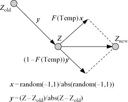
Figure 9.12: Weighted vector sum of previous and random directions for determining the direction to the next simulation point
9.3.2.3 Adaptive Temp coefficient determination
In conventional simulated annealing, the value of the temperature parameter, Temp, is critical in minimising the number of iterations required to find acceptable solutions. Figure 9.13 symbolises the relationship between Temp and the cost function slope. If Temp is too large, global search dominates and iterations are wasted. On the other hand, if Temp is too small, local search dominates and the optimiser gets stuck in local minima. Experience shows that the optimum value of Temp is strongly dependent on the RF circuit topology; i.e. high Temp is required for circuits with steep cost function and vice versa [8]. Greater computational efficiency is achieved by adapting Temp using an estimate of the cost function slope. An implicit relationship between Temp and the cost function slope estimate is shown in (9.7a) below. The adaptive value of Temp is obtained by replacing the random number with a fixed Raccepted, solving the equation for Temp, and averaging as shown in (9.7b).
![]()
![]()
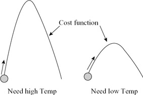
Figure 9.13: The relation between slope of the cost function and Temp coefficient
Figure 9.14 illustrates the computational flow for adaptively determining Temp. For a given circuit topology, experience shows that the estimate of Temp obtained from m iterations within the first optimisation loop (Loop = 1) provides sufficient accuracy for further optimisation cycles.
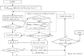
Figure 9.14: The block diagram of adaptive temperature coefficient heuristic
Specifically, all positive cost function differences between iteration points within the first loop are weighted and averaged to estimate Temp. (Of course, the algorithm allows Temp to be estimated from averages over additional loops, if desired.)
While the adaptive Temp algorithm eliminates the need to specify an initial value for Temp, a new empirical parameter, Raccepted, is introduced. It represents the initial probability of hill climbing and ranges from 0.7 to 0.9 depending on the desired optimisation speed. i.e. it determines the balance between global and local search capabilities. Fortunately, a significant advantage accrues from this approach; Raccepted is not dependent on the circuit topology like Temp.
9.3.3 Post-PVT variation optimisation
A key indicator of the robustness of a design is the sensitivity to process, voltage and temperature (PVT) variations. PVT sensitivity should be considered in conjunction with the optimisation algorithm. One approach involves specifying PVT variations as part of the cost function to be optimised. Unfortunately, since the evaluation of PVT variations involves many SPICE simulations at each possible solution point, correspondingly more iterations are required to find acceptable solutions. For example, if 200 circuit simulations are required to obtain PVT sensitivity information at each design point, and 10,000 iterations are required to find an optimum solution before considering PVT variations, the total iteration count grows to 200 10,000 = 2,000,000. The problem here is that PVT variations are being considered for the majority of solutions that are unacceptable to begin with.
A new method for considering PVT sensitivity is post-optimisation PVT analysis wherein PVT variations are simulated for only the accepted solutions. After running PVT Monte Carlo simulations, the average and standard deviation of the resulting cost functions are evaluated and that information is used to possibly redefine an optimum solution. With this approach, the optimum solution may differ from that obtained before post-optimisation PVT analysis.
If, after post-optimisation PVT simulations, the best solution does not meet the specifications, the previously accepted solutions are added to the tunnelling list with the previously unaccepted solutions so that they are not considered further. Figure 9.15 shows the block diagram of the post-optimisation PVT simulation strategy. As indicated, if the optimum solution does not satisfy the specifications after the first optimisation run, the adaptive simulated annealing algorithm is run again. However, note that the simulated annealing algorithm will run much faster during the second optimisation run because of the tunnelling list; it effectively shrinks the design space for each subsequent simulation run by not resimulating known bad solutions.
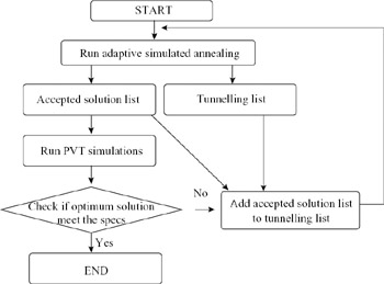
Figure 9.15: Block diagram of post-optimisation PVT variation analysis
9.3.4 Simulation results
A test cost function is chosen as
![]()
Figure 9.10 displays the test cost function versus values of the single design variable, x. It exhibits several local minima and a global minimum. Figures 9.16–9.18 show comparative results between conventional simulated annealing and the new adaptive simulated annealing with tunnelling. The total number of iterations is defined as
![]()
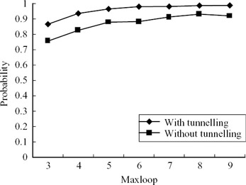
Figure 9.16: Probability of finding the global minimum versus Maxloop for conventional versus adaptive simulated annealing
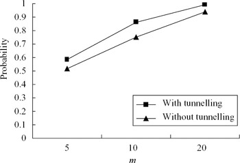
Figure 9.17: Probability of finding the global minimum versus m
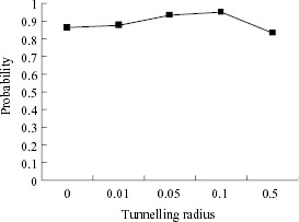
Figure 9.18: Probability of finding the global versus tunnelling radius for conventional versus adaptive simulated annealing
The maximum number of external loop operations, Maxloop, affects inversely the value of the Temp coefficient. That is, if Maxloop is increased, Temp is decreased. m is the maximum number of iterations with the same value of Temp within a given external computation loop. As shown in Figures 9.16 and 9.17, the adaptive annealing algorithm has a higher probability of finding a global minimum givena fixed maximum number of iterations.
Tunnelling employs a coefficient called the tunnelling radius that determines how far the simulation point jumps when tunnelling occurs. This is a critical parameter as shown in Figure 9.18; if the radius is too small, tunnelling occurs infrequently with results similar to conventional simulated annealing. On the other hand, if the radius is too large, unaccepted solutions might obscure the optimum point so that the global minimum is seldom found. Since PVT variations in an IC range over 20 per cent, a value of 5–10 per cent of the parameter value for the tunnelling radius is somewhat arbitrarily chosen.
Tunnelling applied with a simple cost function is shown to be more effective than the conventional hill climbing process in finding the global minimum with a limited number of iterations. Next, tunnelling is applied to the synthesis of an RF power amplifier in fine-line CMOS technology.
|
EAN: 2147483647
Pages: 100