21.4 An RTT Example

We'll use the following example throughout this chapter to examine various implementation details of TCP's timeout and retransmission, slow start, and congestion avoidance .

Using our sock program, 32768 bytes of data are sent from our host slip to the discard service on the host vangogh.cs.berkeley.edu using the command:

 slip %  sock -D -i -n32 vangogh.cs.berkeley.edu discard

From the figure on the inside front cover, slip is connected to the 140.252.1 Ethernet by two SLIP links, and from there across the Internet to the destination. With two 9600 bits/sec SLIP links, we expect some measurable delays.

This command performs 32 1024-byte writes , and since the MTU between slip and bsdi is 296, this becomes 128 segments, each with 256 bytes of user data. The total time for the transfer is about 45 seconds and we see one timeout and three retransmissions.

While this transfer was running we ran tcpdump on the host slip and captured all the segments sent and received. Additionally we specified the -D option to turn on socket debugging (Section A.6). We were then able to run a modified version of the trpt (8) program to print numerous variables in the connection control block relating to the round-trip timing, slow start, and congestion avoidance.

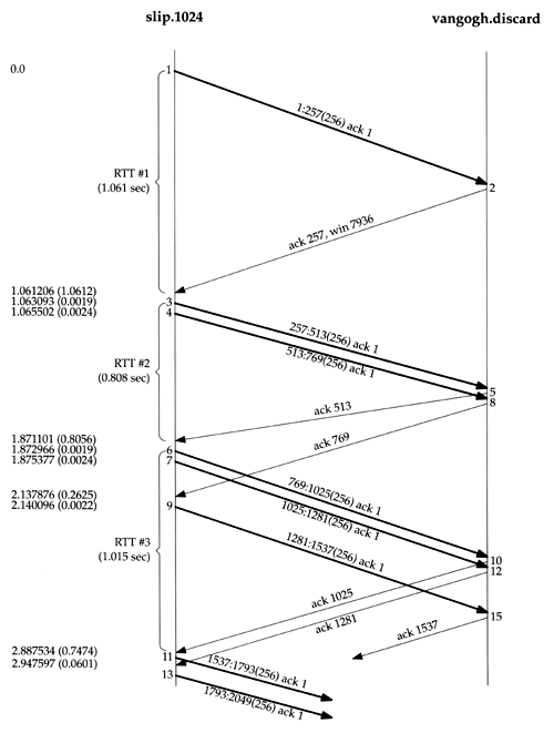
Given the volume of trace output, we can't show it all. Instead we'll look at pieces as we proceed through the chapter. Figure 21.2 shows the transfer of data and acknowledgments for the first 5 seconds. We have modified this output slightly from our previous display of tcpdump output. Although we only measure the times that the packet is sent or received on the host running tcpdump, in this figure we want to show that the packets are crossing in the network (which they are, since this WAN connection is not like a shared Ethernet), and show when the receiving host is probably generating the ACKs. (We have also removed all the window advertisements from this figure. slip always advertised a window of 4096, and vangogh always advertised a window of 8192.)

Figure 21.2. Packet exchange and RTT measurement.

Also note in this figure that we have numbered the segments 1 “13 and 15, in the order in which they were sent or received on the host slip. This correlates with the tcpdump output that was collected on this host.

Round-Trip Time Measurements

Three curly braces have been placed on the left side of the time line indicating which segments were timed for RTT calculations. Not all data segments are timed.

Most Berkeley-derived implementations of TCP measure only one RTT value per connection at any time. If the tinier for a given connection is already in use when a data segment is transmitted, that segment is not timed.

The timing is done by incrementing a counter every time the 500-ms TCP timer routine is invoked. This means that a segment whose acknowledgment arrives 550 ms after the segment was sent could end up with either a 1 tick RTT (implying 500 ms) or a 2 tick RTT ( implying 1000 ms).

In addition to this tick counter for each connection, the starting sequence number of the data in the segment is also remembered . When an acknowledgment that includes this sequence number is received, the timer is turned off. If the data was not retransmitted when the ACK arrives, the smoothed RTT and smoothed mean deviation are updated based on this new measurement.

The timer for the connection in Figure 21.2 is started when segment 1 is transmitted, and turned off when its acknowledgment (segment 2) arrives. Although its RTT is 1.061 seconds (from the tcpdump output), examining the socket debug information shows that three of TCP's clock ticks occurred during this period, implying an RTT of 1500 ms.

The next segment timed is number 3. When segment 4 is transmitted 2.4 ms later, it cannot be timed, since the timer for this connection is already in use. When segment 5 arrives, acknowledging the data that was being timed, its RTT is calculated to be 1 tick (500 ms), even though we see that its RTT is 0.808 seconds from the tcpdump output.

The timer is started again when segment 6 is transmitted, and turned off when its acknowledgment (segment 10) is received 1.015 seconds later. The measured RTT is 2 clock ticks. Segments 7 and 9 cannot be timed, since the timer is already being used. Also, when segment 8 is received (the ACK of 769), nothing is updated since the acknowledgment was not for bytes being timed.

Figure 21.3 shows the relationship in this example between the actual RTTs that we can determine from the tcpdump output, and the counted clock ticks.

Figure 21.3. RTT measurements and clock ticks.

On the top we show the clock ticks, every 500 ms. On the bottom we show the times output by tcpdump, and when the timer for the connection is turned on and off. We know that 3 ticks occur between sending segment 1 and receiving segment 2, 1.061 seconds later, so we assume the first tick occurs at time 0.03. (The first tick must be between 0.00 and 0.061.) The figure then shows how the second measured RTT was counted as 1 tick, and the third as 2 ticks.

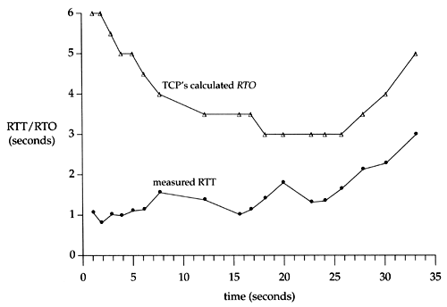
In this complete example, 128 segments were transmitted, and 18 RTT samples were collected. Figure 21.4 shows the measured RTT (taken from the tcpdump output) along with the RTO used by TCP for the timeout (taken from the socket debug output). The x-axis starts at time 0 in Figure 21.2, when the first data segment is transmitted, not when the first SYN is transmitted.

Figure 21.4. Measured RTT and TCP's calculated RTO for example.

The first three data points for the measured RTT correspond to the 3 RTTs that we show in Figure 21.2. The gaps in the RTT samples around times 10, 14, and 21 are caused by retransmissions that took place there (which we'll show later in this chapter). Karn's algorithm prevents us from updating our estimators until another segment is transmitted and acknowledged . Also note that for this implementation, TCP's calculated RTO is always a multiple of 500 ms.

RTT Estimator Calculations

Let's see how the RTT estimators (the smoothed RTT and the smoothed mean deviation) are initialized and updated, and how each retransmission timeout is calculated.

The variables A and D are initialized to 0 and 3 seconds, respectively. The initial retransmission timeout is calculated using the formula

(The factor 2 D is used only for this initial calculation. After this 4 D is added to A to calculate RTO, as shown earlier.) This is the RTO for the transmission of the initial SYN.

It turns out that this initial SYN is lost, and we time out and retransmit. Figure 21.5 shows the first four lines from the tcpdump output file.

Figure 21.5. Timeout and retransmission of initial SYN.

When the timeout occurs after 5.802 seconds, the current RTO is calculated as

The exponential backoff is then applied to the RTO of 12. Since this is the first timeout we use a multiplier of 2, giving the next timeout value as 24 seconds. The next timeout is calculated using a multiplier of 4, giving a value of 48 seconds: 12 — 4. (These initial RTO s for the first SYN on a connection, 6 seconds and then 24 seconds, are what we saw in Figure 4.5.)

The ACK arrives 467 ms after the retransmission. The values of A and D are not updated, because of Karn's algorithm dealing with the retransmission ambiguity. The next segment sent is the ACK on line 4, but it is not timed since it is only an ACK. (Only segments containing data are timed.)

When the first data segment is sent (segment 1 in Figure 21.2) the RTO is not changed, again owing to Karn's algorithm. The current value of 24 seconds is reused until an RTT measurement is made. This means the RTO for time 0 in Figure 21.4 is really 24, but we didn't plot that point.

When the ACK for the first data segment arrives (segment 2 in Figure 21.2), three clock ticks were counted and our estimators are initialized as

(The value 1.5 for M is for 3 clock ticks.) The previous initialization of A and D to 0 and 3 was for the initial RTO calculation. This initialization is for the first calculation of the estimators using the first RTT measurement M. The RTO is calculated as

When the ACK for the second data segment arrives (segment 5 in Figure 21.2), 1 clock tick is counted (0.5 seconds) and our estimators are updated as

There are some subtleties in the fixed-point representations of Err, A, and D, and the fixed-point calculations that are actually used (which we've shown in floating-point for simplicity). These differences yield an RTO of 6 seconds (not 6.3125), which is what we plot in Figure 21.4 for time 1.871.

Slow Start

We described the slow start algorithm in Section 20.6. We can see it in action again in Figure 21.2.

Only one segment is initially transmitted on the connection, and its acknowledgment must be received before another segment is transmitted. When segment 2 is received, two more segments are transmitted.