3.2 CODING
| Codes can be concatenated with the basic DMT system in ADSL to improve performance, nominally by as much as 6.5 to 7.5 dB with random background crosstalk and line noise, and by a larger amount with impulsive disturbances. At the time of first ADSL standardization, a concatenated coding system ( trellis code with outer interleaved Reed Solomon) was mandated . That system has considerable flexibility and thus, while implemented without full ability to understand codes of the future, fortunately can be used to provide more transmission robustness than originally anticipated. The designer needs to know only how to best decode that earliest specified system. Present-day knowledge allows high coding gain of 6 “8 dB with a more complicated decoder than originally planned. However, the gain versus complexity improvement of a better decoder may not merit the effort. Even the most modern of codes and decoder methods can be implemented as a fraction of the digital-signal processing on ADSL digital chips that today cost less than $5/line on average to make. An aspect of coding not addressed in previous work [1] is the proper loading of the ADSL DMT modem and the proper swapping mechanisms when codes are used. This is addressed in Section 3.3. Also of importance in coded DSL is calculation of performance somewhat more precisely than simple approximations, which can be inaccurate, as well as improvement of this performance level in the presence of AWGN. Section 3.2.1 addresses performance calculation and advanced codes. Also of importance is impulse noise. Section 3.2.2 adds to previous models and understandings of impulse noise in [1] and also provides a method for analysis of any impulse in terms of performance loss. Section 3.2.3 discusses interleaving and its use. 3.2.1 High-Level Analysis and Advanced Codes (and Pointers for Decoding)Trellis codes and Reed-Solomon (RS) codes for ADSL were detailed in [1]. Section 3.3 details exact coding gains of the RS code, while the trellis code adds approximately 1.5 dB to the gain of the RS code, which makes the total coding gain about 5 to 5.5 dB for white Gaussian noise with hard decoding of the RS code and Viterbi decoding of the trellis code. Soft or iterative decoding of the RS and trellis together could lead to 7 “8 dB of coding gain. Impulse noise is discussed in the next section. Since early standardization, more easily implemented powerful coding systems have come into greater acceptance and understanding. These turbo and low-density parity check ( LDPC ) codes have longer block lengths (or more exactly greater memory span) than the trellis code, and have been proposed as optional replacements for the earlier trellis codes. [4] The advanced codes follow the basic outline of information theory that suggests more random structure to the encoder is usually good if the block length is sufficiently long. Turbo codes generally achieve the randomness through interleaving two simpler convolutional (or in effect in ADSL, trellis) codes. LDPC codes are based upon random construction of a parity matrix. The main improvement over trellis codes is achieved by implementation of the decoder through suboptimal iterative calculation/ approximation of the log- likelihood of the probability distribution for each bit transmitted. Such algorithms almost always perform very close to optimum with a complexity far less than traditional exhaustively searching detectors or soft decoding of the RS code, and are often easier to understand than optimum decoders, but do require numbers of decoder operations well in excess of the trellis Viterbi decoder alone. The February 2001 issue of the IEEE Transactions on Information Theory [19] and the May 2001 issue of IEEE JSAC [20] are dedicated to these newer codes and contain much information. This chapter outlines performance gains of two specific proposals for ADSL by AT&T [4] and IBM [5], turbo and LDPC, respectively. The reader is also referred to the Web site [21] for worked examples of encoders and decoders based on these two codes in a forthcoming academic textbook .
Turbo and LDPC codes are binary and thus do not uniformly map bits to an ADSL DMT symbol, which uses multilevel constellations on each tone that may vary the number of bits/tone from 0 to 15. Lauer [22] found the nonuniformity to be of little consequence and that straightforward mapping of the encoder output bits through the constellation mapper for the DMT modulator tones with proper construction of the a priori likelihoods from the corresponding receiver FFT outputs allows achievement of the nominal gain of the code. For construction of the likelihoods necessary to initiate iterative decoding for such systems, see the examples at the Web site [21]. Such normal gain is typically about 7 dB, but is a little larger on tones with smaller numbers of bits and a little smaller on tones with a larger number of bits. However, such an approach has three drawbacks for ADSL:
Several researchers at AT&T [4] studied these issues carefully and proposed a solution that involves use of a binary rate-one-third turbo code, use of a special interleaver designed to match the ADSL frame structure and to eliminate turbo-code error floor effects, and variable puncturing of parity bits according to the number of bits per symbol to handle any constellation size . The code can thus be characterized as two-dimensional in the same sense as the existing ADSL trellis code is four-dimensional. The code has a gain at 2 bits per symbol of nearly 9 dB, which drops to about 6.2 dB for the largest constellations, making the gain about 7 dB overall. The code is based on two interleaved uses of an eight-state convolutional code of rate one-half with generator Several IBM researchers [5] have instead proposed a class of LDPC codes based on array codes that only encode the lowest 1 or 2 bits per dimension, thus simplifying the decoder. The output bits of the coder selects cosets in the same way that trellis code encoders do (see [1]), that is, in one dimension with exclusively square constellations. Special cases for small constellations are enumerated in [5]. The intrapartition distance is thus 12 to 18 dB, well above that of the code. The structure thus allows a lower complexity decoder and the same gain against AWGN, which is again 6 “7 dB for the LDPC code. Impulses that exceed the intrapartition distance will cause errors and thus force the use of external FEC, but that is nominally implemented in any case. The advanced encoding architecture for any of the cases is illustrated in Figure 3.3. The dual latency structure of ADSL is preserved with only short-block FEC applied in the "fast" path and both advanced coding (LDPC or turbo) and interleaved FEC applied in the " interleave " (or "slow") path. Although no advanced codes have yet been agreed for standardization, this area is likely to be one of advance in the G.dmt.ter standard of the future in the ITU. Decoding is more computationally complex than hard RS decoding combined with Viterbi-trellis-code decoding, and the reader is referred to [21] and [23] for detailed information on decoding and exact analysis. Figure 3.3. Advanced coding architecture. 3.2.2 Impulse Noise CharacterizationImpulse noise has become one of the dominant issues in ADSL deployment, affecting range and reliability for all data rates. With the increase in ADSL deployments, several phone companies have studied the modeling of impulses and have derived models to help in qualification of service. These models are also useful for testing and design of better ADSL modems. This section summarizes models and improves upon the art in terms of providing models that could be used in testing as well as in design of better ADSL modems. Figure 3.4 illustrates an impulse generation mechanism. There are three key elements in the generator:
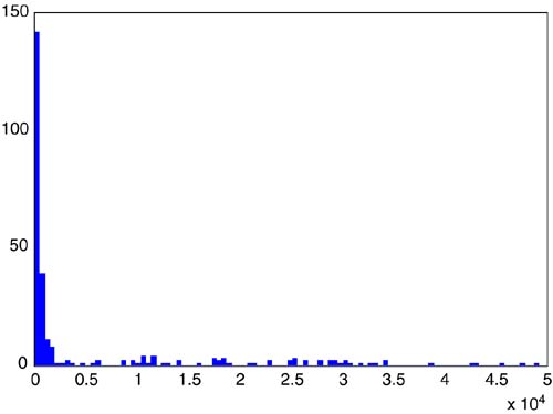
Figure 3.4. Impulse generation mechanism. The waveform storage may have measured impulses or mathematically modeled impulses stored, perhaps several of them. (Alternatively, the waveforms may be statistically generated.) Each stored waveform may have a certain probability of being selected when the generator extracts the next impulse from storage. The time of extraction is measured from the termination of the last impulse generated and is determined by the interimpulse-delay generator or "delay to next impulse" in Figure 3.4. The delay generator is reset each time the last impulse is finished transmitting. The impulse waveform is scaled by the amplitude generator. The amplitude is selected randomly from a distribution of amplitude or possibly fixed at some constant, depending on the specifics of the impulses that the telephone company desires to test (or that the ADSL designer desires to analyze). Sometimes a random amplitude is selected for each stored sample of the impulse in addition to a gross gain applied to the entire impulse. Impulse Amplitude DistributionThe amplitude box in Figure 3.4 simply scales the impulse waveform by some (usually randomly chosen ) constant. Of interest is the distribution for the constant, which is often randomly selected each time a sample of an impulse is generated. France Telecom [6] provides histograms of various impulse-noise measurements. In particular, Figure 3.5 (repeated from [6]) illustrates a histogram of impulse energy. Small-energy impulses have the highest probability, whereas very large impulses tend to be less probable. One can see that about 90 percent of impulses have a duration of less than 250 µs (see also Figure 3.7) and have amplitudes of less than about 10 mV. However, there are a small fraction of impulses that may also have very high amplitudes. Thus a theoretical model that perhaps somewhat conservatively overestimates the probability of large peak impulses may be useful in making theoretical projections based on the energy histogram in Figure 3.5. Impulses with amplitudes greater than 200 mV are very unlikely . For impulse sizes below 10 mV, the probability grows roughly linearly with the log of the peak voltage (or energy, assuming the logarithm of the two are linearly related ). Figure 3.5. Impulse energy histogram (horizontal axis is dB in Watts/Hz). Courtesy France Telecom [6]. Figure 3.7. Impulse duration histogram (horizontal axis is m s, to 50 ms spanned ). Courtesy France Telecom [6]. The author has empirically guessed a distribution for the energy from the histogram in dBm/Hz. which has a discontinuity at “75 dBm/Hz but projects 90 percent of impulses below this energy level and 10 percent above. A distribution such as the one above, even given it is not perfect, allows projection of ADSL error statistics theoretically. This particular model does not predict a large number of tiny impulses. It is useful only for a gross gain per generated impulse and not for each sample of an impulse. This model would be used when a set of a few impulses is stored and generated as in Figure 3.4. A more elegant approach to impulse energy characterization has been provided by the work of Henkel and colleagues [24],[25]. Two distributions are provided that are shown [25] to model well measurements by British Telecom and Deutsche Telekom. The first model is a simple exponential distribution [5] given by
which has mean zero and variance Figure 3.6. Exponential probability distribution for impulses. The alternative Weibull distribution offered by Mann et al. [25] is This distribution also overemphasizes small values excessively, but well approximates the tail of the impulse distribution because of the same exponential dependence. Generation of this distribution is described in [8] and can be tailored to provide a given autocorrelation function also. However, the generator in Figure 3.5 (unlike the structures in [25] and considered by ETSI) does not need specification of the autocorrelation function of the impulse because several impulses can simply be stored and then selected each with some individual probability, following more closely the impulse classification in [7] into a handful of representative shapes . Various phone companies have measured the values for A in the exponential distribution and a ,b in the Weibull distribution. We list a few here, partially repeated from [7]:
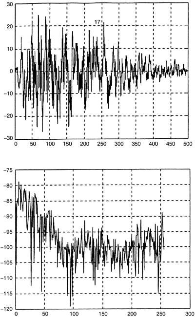
North American phone company impulse measurements were not available at time of writing. Impulse Duration DistributionFigure 3.7 illustrates a histogram of measured impulse durations. Clearly some impulses are very long, but have low probability of occurrence. Indeed, many impulses are very short, less than 100 microseconds in duration. These short impulses will most often have small amplitudes, and indeed it is possible for many small impulses to follow each other closely in time without disruption of service. The approach of standards groups so far has been to define models that are accurate in the tails of probability distributions, that is, that big impulse samples occur infrequently and last a long time whereas small impulse samples of little consequence can occur often. If the tails are modeled correctly by testing or analysis, then the frequent small impulses may not significantly alter performance projections (and indeed match measurements anyway as evident from Figure 3.7). Extremely long impulses typically have energy concentrated in a small number of frequency bands. Specifically in the model of Figure 3.4, the impulses are separated by a delay. Figure 3.8 illustrates a model of the generation of the inter-impulse delay. Basically, the generator contains a 2-state machine (Markov model) with one of the states being that the next impulse will occur in less than 1 ms and the other state being that the next impulse will occur after more than 1 ms of delay. Each time an impulse is sent, the state machine can make a transition, either to stay in the same state or to change states. Figure 3.8. State transition diagram for interimpulse delay. The probability that a short delay is followed by another short delay is written as p s/s whereas the probability of a long delay following a short delay is p l/s . The probabilities can be summarized in the matrix and the so-called Markov distribution for the probability of short delays and long delays is determined by There are two distributions for the interimpulse delay t : with typical l = .16 and with typical a = 1.5 and t in ms. The first distribution produces with small probability delays that can exceed 1 ms, and these delays are discarded and the random selection procedure cycled again until a delay less than 1 ms occurs. The second distribution exists from 1 ms to infinity. Both can be easily generated from a uniform random variable u on the unit interval [0,1] by the transformations and respectively. A 2x2 matrix is then provided with upper left entry corresponding to the probability that a short interarrival time is followed by a second short interarrival, the lower right corresponding to long followed by long. For instance, ETSI uses a model based on British measurements: which (e.g., for the default) means that 80 percent of the time a short interarrival occurs, the next interarrival is also short, and the other 20 percent of the time the next impulse is more than 1 ms away and has the probability of interarrival given by the long distribution. Similarly, 60 percent of long-interarrival impulses are followed by long interarrival impulses. The default matrix provides that one-third of the impulses are separated by at least 1 ms, whereas the other two- thirds are very close together. Most samples of any impulse are again small, so even very many samples of those impulses with long interarrival times between them are small. The possibility of two large impulses in a row is thus very small, but not zero. France Telecom has found yet another model that is more characteristic of their network and is Impulse WaveformsOne particularly in-depth study by C. Collobert and colleagues at France Telecom [7] has found after looking at enormous volumes of ADSL impulse data that impulses can be classified through the use of neural networks into categories that have similar profiles in terms of a cumulative spectral density. FT was able to find five classes that well characterized all their impulses. Each ADSL class is then characterized by a single impulse for test purposes, but the amplitude of that impulse may be nominal (0 dB) or increased to 6 dB larger, and decreased -6, -12, -18, and -24 dB lower in amplitude. An impulse used in one of the ADSL classes derived by FT appears in Figure 3.9. Here the amplitude of the impulse is very large, corresponding to a scaling with rare occurrence in the model of Figure 3.4. The associated frequency spectrum is also plotted in Figure 3.9. Note the impulse is large and long and could be expected to cause difficulty for transmission. With only a few classes, one could evaluate the probability of the different classes empirically (or perhaps adaptively in real time) and then complete the model of Figure 3.4 by storing representative impulse waveforms in the impulse-waveform-storage box. By contrast, in statistical generation using the exponential or Weibull distributions, the autocorrelation of classes of impulses may be stored, and the impulses are generated using these autocorrelations [25]. Figure 3.9. France Telecom's "Imp" class impulse (horizontal axes in m s and ADSL DMT tone index, respectively, vertical axes in mV and dBm/Hz). Others have tried to create mathematical models for the impulse. For instance, Reference [1] describes impulses and a characterization published by BT known as the Cook Pulse. The Cook Pulse has a discrete-time model when sampled at interval T, or equivalently at times kT, that is, zero at time k = 0, and otherwise is Approximately 45 percent of the impulse energy is in the peak sample and the rest decays with time. Longer impulses tend to have larger peak voltages, and the peak voltage also increases with increased bandwidth use (sampling rate, 1 /T ) of the DSL system, roughly as In recent years , many phone companies have further studied impulse noise and found the Cook pulse to be insufficient in characterization. Thus other models have been attempted. One such model was proposed in [25] for ETSI specification. This model essentially models the impulse as an exponentially windowed sinusoid with the exponential decay of the window and the frequency of the sinusoid each determined by random selection from a Guassian distribution. The duration of the window is also random and determined by selection from a convex sum of two log-normal distributions. The model for the autocorrelation function of the impulse is thus where g and b are the Gaussian parameters. The parameter g is selected to be one of 3 Gaussian random variables as shown in Table 3.1, whereas the window parameter b is selected from one of four Gaussians characterized by the randomly selected length of the impulse as shown in Table 3.2. Table 3.1. g Values
The distribution for the length of the impulse (equivalently the length of the exponential window) is where the customer premises parameters are B = 1, s 1 = 1.15, t 1 = 18 µ s , and thus the second term above is zero, and the CO parameters are B = .25, s 1 = .75, t 1 = 8 µ s, s 2 = 1.0, t 2 = 125 µ s .This model is likely less representative, and certainly much more complex to implement and understand, than Collobert's representative waveforms in [7]. ETSI is now evaluating the France Telecom impulse-class model. Probability of Error Analysis with Impulse NoiseThe authors would especially like to thank Dr. Wei Yu and Mr. Daniel Gardan for inputs to this section. ADSL uses Reed-Solomon codes to provide coding gain and also to mitigate impulse noise disturbance. The RS code is a block code of block size up to 255 based on GF(2 8 ) (or bytes). An RS code word can therefore be up to 255 bytes long (in ADSL systems). The RS code word boundary is aligned with the DMT symbol boundary. Because of the rate adaptive nature of a DMT system, the number of bits in each DMT symbol varies depending on the data rate. ADSL [3] allows a variable number (1, 2, 4, 8, or 16) of DMT symbols for each RS code word. ADSL also allows an even number of parity bytes (up to 16) to be included in an RS code word. The decoder is able to correct up to half as many error bytes. In order to take full advantage of the error-protecting ability from RS code, it is important to correctly choose the number of DMT symbols per RS code word and the number of parity bytes included in each code word. From a pure error-correcting point of view, for the same amount of parity overhead, it is always the best to have as many DMT symbols in an RS code word as possible. For example, a system that includes 8 DMT symbols and 16 bytes of parity for each RS code word performs better than a system that includes 4 DMT symbols and 8 bytes of parity for each RS code word. This is because the former system can correct at least as many errors as the latter system. A longer RS code word means longer delay, and possibly more decoder complexity. The analysis here concentrates on reducing the impact of impulses as best as is possible, and will therefore include as many DMT symbols per RS code word as possible for impulse protection, necessarily enduring delay. Then it only remains to decide how many parity bytes to include in each RS code word. Table 3.2. b Values
In most cases, the maximum error-correcting protection against Gaussian noise when the system operates near capacity is obtained when the parity overhead is approximately 6 to 10 percent [18], which is about 16 parity bytes in 128 “256 bytes. The RS code word length depends on the number of DMT symbols per RS code word; thus, it depends on the system data rate. (A framing overhead of 128 kbps is assumed here.) For example, at 608 kbps, each DMT symbol is about (608 + 128)/4 = 184 bits = 23 bytes long. So, up to 8 DMT symbols can be grouped into an RS code word. Assuming 16 bytes of parity are inserted, the resulting RS code word is 23 · 8 + 16 = 200 bytes long. At 1.216 Mbps, each DMT symbol is about (1216 + 128)/4 = 336 bits = 42 bytes long. So, up to 4 DMT symbols can be grouped into an RS code word. Again assuming 16 bytes of parity, the code word length is 42 · 4 + 16 = 184 bytes long. At 2.048 Mbps, each DMT symbol is (2048 + 128)/4 = 68 bytes long. So, 2 DMT symbols are grouped into an RS code word, resulting in a code word length of 68 · 2 + 16 = 152 bytes. Assuming 16 bytes of parity, the RS code is able to correct up to 8 bytes of error. When more than 8 errors occur, the Reed-Solomon decoder will either decode to a false code word, in which case nearly all the bytes (or half of the bits) are incorrect; or the decoder will declare decoding failure, in which case the original code word is unchanged so the output has the same number of error bytes as before. The following calculation shows that decoder failure is a much more likely possibility: The RS code operates on GF(256). The total number of length -256 valid code words is 256 240 . (This is because the 16-byte parity is to be added to any 240-byte message.) For a correctable error to occur, at most 8 bytes can be in error. These errors can be located in Many ADSL receivers use erasures for impulses. A simple erasure mechanism that works very well is to compare the sum of squared differences between tone decoder slicers' outputs and inputs. Nominally this sum is nearly zero if there is no impulse. When this sum exceeds a threshold, all bytes in the DMT symbol are "erased" ( marked ). The RS decoder can then correct erased bytes (twice as much). Even in this case, failed RS decoding is easily detected . The following analyzes the coding gain of an RS code in an AWGN channel. In an AWGN channel (or a channel with a well-designed equalizer), the probability of error for each byte is approximately the same. Let Pe denote the probability of a byte error. When Pe is small, the probability of code word error is closely approximated by the probability that 9 byte errors occur. When 9 byte errors occur, the Reed-Solomon decoder will declare decoding failure, so the total number of error bytes will be 9. For each byte error, the most probable channel defect is that a single bit is likely to be wrong. So the probability of bit error in the code word is 9/200/8 = 4.4 · 10 -3 , when a decoding error occurs. Because the required probability of bit error is 10 -7 , the required probability of code word error is 10 -7 /4.4 · 10 -3 . In this case, a 608 kbps ADSL system with 200 bytes per RS code word needs to satisfy : Thus the uncoded system needs to have Pe = 0.0065 for each byte to attain an overall probability of bit error 10 -7 . Since the probability of byte error is 0.0065, the uncoded probability of bit error is then [6] 0.0065/8 = 8.1 · 10 -4 . The gap for QAM at P b = 8.1 · 10 -4 is found by noticing 2Q(10.5dB) = 8.1 · 10 -4 . So instead of requiring the argument of the Q-function to be 14.5dB, with coding, only 10.5dB is needed. In other words, coding provided a gain of 14.5dB - 10.5dB = 4.0dB. This is the coding gain for a 608 kbps system with 8 DMT symbols per RS code word and 16 parity bytes. This (raw) coding gain does not take the extra parity overhead into account. In reality, having 16 bytes of parity for every 8 DMT symbols translates to an extra 64kbps coding overhead. The loss in dB for the overhead is 64/(256 · 4) = 1/16 or .4 dB so the actual coding gain is 3.6 dB. This method of calculating the RS coding gain is more accurate than assuming 3dB coding gain for all systems. One needs to exercise caution in impulse analysis as opposed to AWGN-analysis in Section 3.3.5 ”here the probability of bit error is in the range of 10 -4 whereas in Section 3.3.5, the same probability is computed under an assumption of 6 dB margin at 10 -7 and can thus be expected to be higher (coding gain is constant only as probability of error gets small, or SNR is high, which is not true in this section). Use of erasures does not improve performance with Gaussian noise.
Probability of Error Calculation for ImpulsesUncoded SystemThe filtered impulse samples are treated as a deterministic signal. Its interpolated and resampled version is passed to an FFT demodulator. The resampling rate is 2.208MHz, and the FFT size is 512, representing 512 real dimensions in a DMT symbol. The noise samples contained in the cyclic prefix are discarded. The output of the 512-FFT is then combined into 256 complex samples, representing the real and imaginary parts of the impulse noise in each tone. The complex disturbance is the perturbation to the constellation caused by impulses. The perturbation decreases the minimum distance between constellation points, and hence increases the probability of bit error. Strictly speaking, the increase in probability of error caused by impulses depends on the constellation size (because the boundary points are less susceptible to impulse disturbance than points in the middle of the constellation.) A simplification assumes all QAM points have exactly four nearest neighbors, and four next- nearest neighbors, and computes the probability of error based on these neighbors. Figure 3.10 illustrates the computation. Figure 3.10. Illustration of impulse analysis Pe calculation. In Figure 3.10, suppose that the constellation point X is being sent. Without impulse, the probability of error in the presence of AWGN is closely approximated by Pe = 4 Q(d/ 2 s ) , where d is the minimum distance between constellation points, and s 2 is the AWGN noise variance. The coefficient 4 represents the four nearest neighbors of each constellation point. When the system is disrupted by an impulse, the impulse is regarded as a deterministic signal, shown in the diagram as an arrow from the original constellation point X to the new location Y . If Y is outside of the decision region, an error is almost certain to occur. In this case, P e = 1. If Y is inside of the decision boundary, the probability of error is computed by summing over the probability that the point Y may be confused for each of the neighbors: where d i are the distances between Y and its neighbors A, B, C, D , and E . Strictly speaking, summing the probability is only valid when the error events are mutually exclusive. The above formula is thus an upper bound. Following the preceding calculation, the probability of symbol error for each tone may be calculated separately. Because each tone carries different number of bits, the average probability of bit error is computed as where P i is the probability of symbol error on each tone, and b i is the number of bits carried on i th tone. Coded System In a coded system, the minimum distance between constellation points is smaller than an uncoded system because a coded system partially relies on the error correcting code to compensate for the smaller dmin. The goal is to compute the expected number of error bits when an impulse occurs. Evaluation first requires translation of the probability of bit error into the probability of byte error, because RS code works on bytes. Every 8 bits are grouped into a byte, and the probability of byte error The performance measure of interest is the expected number of byte errors. When there is no coding, the expected number of byte errors is just the sum of P byte (k) , where P byte (k) denotes the probability of byte error in k th byte. When an FEC is implemented, the probability events with fewer than nine errors are successfully corrected, so an expression for the average number of byte error is: [7]
The above expression is relatively easy to compute. Although enumerating all 8-byte errors in a 200-byte code word involves summing over Table 3.3. Interleaving Parameters on an ADSL Modem
InterleavingIt is interesting to note that major service providers have indicated that approximately 99 percent of ADSL lines are operating without interleaving (fast mode). This is motivated by the desire to provide low latency transport. Many of the 1 percent of lines with interleaving use the interleaved mode to increase line reach or attempt to resolve service troubles. ADSL allows RS code word to be interleaved with an interleaver depth of 1, 2, 4, 8, 16, 32, or 64. If the interleaver size is D, byte i in an RS code word is delayed by ( D “ 1) i byte transmission times. The interleaved version is sent over the channel and is corrupted by impulses. The deinterleaved version is decoded, so, in effect, the number of corrupted bytes decreases by a factor of D. To calculate the effect of interleaving on isolated impulse, analysis can assume that impulses are far enough apart so that after deinterleaving, no two impulses occur in the same code word. Table 3.3 summarizes typical interleaver parameters for three data rates. Impulse AlignmentIn real systems, impulse may occur at any time instant. So an impulse typically spans more than one DMT symbol, and could also span more than one RS code word. This effect needs to be taken into consideration in any simulation. For results of simulations using methods like those described here, see [6]. Often detailed uses of this type of analysis for specific impulses is held secret by the service providers who endeavor to compute them. 3.2.3 Interleaving and Decoding ImprovementsInterleaving and deinterleaving are described in [1] for ADSL and allow an interleave depth, D, of up to 64 code words. Up to sixteen DMT symbols per code word are also allowed at very low data rates, so that a delay can be up to 256 ms. Fast path delay is limited to 2 ms, and the number of symbols per code word is forced to one as is the interleave depth. Minimum delay is desirable for interactive applications like voice or games , although realistically a user does not notice (on an echo canceled network link) delays of less than 100 ms (no matter what standards and experts say). [8] Thus it is often advantageous to use the maximum delay and corresponding interleave depth of sixty-four whenever possible for extra impulse protection. At higher speeds where the number of symbols per code word is four or less, the delay is inconsequential to most applications. More important though is that increased delay leads to increased buffering of data throughout the network, which then can impose a more stringent delay constraint on the ADSL link. This delay has nothing to do with applications, but instead is caused by insufficient buffer-size decisions in other parts of the network or protocol used. Network designers of the future will consider the impact that better ADSL end service will have on their sales and revenues and understand that excessively tight delay constraints on the DSL modem is quite counterproductive for their overall objectives, and otherwise arbitrarily imposed by poor network choices. Also, reference [29] has recently made significant progress in mitigating all impulses with very low latency.
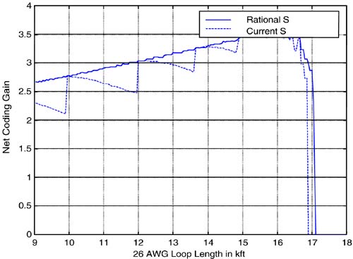
This area still remains one of active interest and study today as to how to obtain the best possible impulse-noise rejection with the least delay. Fortunately, DMT offers a theoretical advantage of 24 dB (and a measured advantage of about 10 dB) in impulse-noise rejection with respect to other non-DMT-based DSLs, making the trade-off somewhat more palatable for ADSL than for other non-DMT DSLs. 3.2.4 Impulse-Cognizant Loading and Erasure MethodsA strong feature of RS codes is their capability to correct double the number of errors if the location of the error bytes is known. This is called erasure decoding, and is very useful for impulse noise. Clearly, such a capability also allows halving the interleave depth (or halving the delay and the amount of memory required for implementation) for a given level of impulse protection. Several ADSL modem manufacturers exploit this capability. Impulses must be detected for erasures, typically of all bytes in any DMT symbol known to be simultaneous with an impulse. As mentioned earlier, an easy impulse-defect metric is simply the sum of the squared tone-slicer errors. Reference [29] is a very recent study of 11,000 France Telecom impulses that uses an erasure RS decoder to remove all errors from all impulses with less than 5 ms latency. It is the first public report of successful use of erasures. Cioffi suggests that recent soft-decoding algorithms with trellis coding can be applied; for instance, the well-known SOVA method [9], soft-output Viterbi algorithm. These methods are more complex than the usual Viterbi detector, but retain a reliability indicator for the selected bits/symbol strings that can be simply processed to provide a reliability indicator for each byte input to the following FEC decoder. This may allow more than impulse-type erasure. In normal operation with 6 dB margin, the reliability indicator will be excellent and will suggest no errors are being made. When impulse or other non-Gaussian noise is present, the reliability indicator will be poor, suggesting that many errors are being made. There is an independent reliability indication for every DMT tone symbol (or at least every two symbols in the four-dimensional code). The reliability indicator for a byte is essentially the sum of all symbol reliability indicators for the symbols that contribute bits to that byte. This is an unusual use of SOVA, but consistent with iterative decoding methods that heavily and productively use SOVA for AWGN disturbances. To further this concept, recent turbo and LDPC code proposals for ADSL (see Section 3.2.1) may find acceptance. In these proposals, the trellis code is replaced by a more powerful turbo/LDPC, and the reliability indicator is inherent in the decoding methods used for those codes. While already having 6.5 dB or more of coding gain, and better performance against impulses themselves , the reliability indicator of these codes can also be passed to the FEC decoder and used as an erasure indicator. The probability of false indication of an erasure is far less with these advanced decoding algorithms (such as SOVA or iterative log-likelihood construction for LDPC), and thus they offer an enormous possible improvement for impulse noise rejection. This area is still under study by several groups and likely to be one of the improvement areas of ADSL in the future, but verifiable results have yet to be published. Another method for improving impulse reliability that is simpler, but reduces data rate, is impulse-cognizant loading. In impulse-cognizant loading, the distribution of energy of the impulse is either known or estimated on-line. Most impulses while generally perceived to be wideband, do not cover the entire frequency spectra equally (indeed the reason why the normal 24 dB [= 10 log 10 number of tones] advantage of DMT is more like 10 dB in practice). However, often lower frequencies are affected with larger amounts of energy. Thus, the margin for the lower frequencies can be increased (while upper frequencies, or more generally those known to be relatively unaffected by impulse energy, can have their margins in turn decreased). This procedure either reduces data rate or overall margin against Gaussian noise, but can improve margin against impulse noise. Such a procedure can dramatically reduce the amount of interleaving necessary for the same-level impulse protection (perhaps by as much as a factor of three or four) for perhaps the cost of several hundred kilobits in aggregate maximum-achievable data rate or throughput, which may be an acceptable trade in many cases (especially if the implemented data rate is already well below the maximum achievable). The difficulty is knowing what frequencies/tones are disturbed most on any given line, which may have many sources of impulses. Again, the soft-information/reliability-indicator of more advanced codes may create opportunity in the future to do greater on-line characterization of impulses on any given line in the receiver, thus creating the opportunity for frequency-selective loading. The authors expect impulse rejection methods to improve significantly in the future, and likely the data rates of ADSL in deployments will be increased in many regions from 500 “800 kbps downstream rates (which are very conservative largely because of impulse noise and a perceived need for low latency) to 1.5 Mbps on 4-mile lines. Theoretically, impulses have very little energy over all time, even over short intervals in time, and thus should not dramatically reduce performance. To induce huge margins on DSL service to protect against impulse problems is therefore unnecessary and inhibits the long-term capabilities and revenues of DSL. 3.2.5 Decoupling of ADSL Frame and CodeDecoupling of the ADSL framing from the DMT symbols allows a greater continuum of FEC parameters and has been incorporated into the lastest ADSL standards drafts. New FramingThe ITU second-generation ADSL recommendations G.992.3 and G.992.4 [3] include a new reduced-overhead framing mode for ADSL. Earlier ADSL modems supported four framing modes having different amounts of minimum overhead with one or two latency paths. These paths can be configured to have different overheads and thus have different framing efficiencies. With an RS code word enabled, the minimum overhead is 64 kbps or higher, corresponding to 2 bytes of parity per DMT symbol. This causes substantial framing inefficiencies at low-line rates such as 224 kbps or lower, quite typical in the upstream directions on long loops. The same framing inefficiency also existed for downstream link on long loops . The earlier standardized ADSL framing overhead used at least one overhead byte per frame and only an integer-ratio choice of R (RS code word parity bytes) and S (Number of DMT symbols over which the RS code word spans) parameter values for RS code word. The new ADSL standards make appropriate adjustments in these parameters and can minimize these inefficiencies . In addition, the early standardized framing was byte aligned and required the DMT symbols to carry an integer number of bytes, causing additional inefficiencies up to 28 kbps. Together, up to 92 kbps minus the required minimum overhead is now available to improve user payload in the new framing. The new standards achieve this reduction by removing the integer constraint on the ratio of R/S and allowing the overhead to be configurable to smaller values than 32 kbps. This, in effect, also removes the constraint of the DMT symbols to carry an integer number of bytes or the line rate to be an integer multiple of 32 kbps. These modifications can provide very significant improvements toward the net data rate of the modem. For example, by configuring the current framing to have a 4 kbps overhead and 4 kbps RS overhead, ADSL can avail 88 kbps toward the net data rate just because of the improved framing. Allowing S to be a rational number further helps optimize the coding gain on all loops. The granularity of the S does not permit maximized coding gain on all loop lengths. The dotted curve in Figure 3.11 shows the effect of current S values as a function of 26 AWG loop length with link latency less than or equal to 16 ms. Because of coarse granularity in current S values, there is a reduction in net coding gain of the modem as a function of loop length and then a jump back to optimum coding gain as the next optimum S value becomes available. On the other hand, rational S values optimize the coding gain on all loop lengths. The maximum net coding gain advantage is about 0.64 dB in this example. This advantage varies on different loops but rational S always performs equally or better. Figure 3.11. Net coding gain produced by new ADSL framing proposal (see [6]). There is a direct relation between the line rate and the coding gain. For example, an increase in coding gain corresponds to a certain amount of line rate increase on a given loop. After taking into consideration the overhead associated with the coding scheme, this transforms into a net data rate increase. Thus, increase in net data rate due to increased framing efficiency would also correspond to a certain amount of coding gain. In other words, increased framing efficiency corresponds to increased coding gain. 1-Bit ConstellationITU Recommendations G.991.3 and G.992.4 also include provisions for 1-bit signal constellations. Earlier ADSL modems do not support the use of 1-bit constellations on subcarriers. The 1-bit constellation allows the use of those subcarriers that do not have sufficient SNR to support the 4 QAM constellation but sufficient to support 2 QAM. This helps increase the total capacity of the ADSL modems without a significant increase for implementation complexity. One-bit carriers also simplify swapping, as in Section 3.3. In a theoretical simulation of the ADSL modems on ISDN # 7 loop with 24 HDSL crosstalk, the capacity without the use of 1-bit constellation was 468 kbps downstream and 168 kbps upstream, respectively. The same improved to 596 kbps downstream and 196 kbps upstream, respectively, when the use of 1-bit constellation was enabled. This advantage would vary among different loop and crosstalk scenarios, but, in general, there would be some increase in capacity due to the use of 1-bit constellation. The implementation of transceivers with 1-bit constellation must also address the bit assignment for trellis coding. Rate AdaptationThe transmission environment encountered by ADSL modems is not long-term stationary. Crosstalk noise changes as the other users in a binder group connect and disconnect modems. Other noise changes are due to radio transmitters transmitting more or less power. The signal attenuation changes with time of the day due to changes in cable temperature. A service margin of 6 dB in the current ADSL modems should provide protection against changes due to these factors for all but the most extreme cases. However, this results in many lines operating with far more margin than necessary, and some lines operating at some times with virtually no margin. Rate adaptation in the improved ADSL modems would allow for dynamic (in-service) changes in the line rate without losing payload data. This is possible because of the new framing that allows transparent reconfiguration and a change in the modem line rate through a message-based line reconfiguration protocol, which is run over the ADSL overhead channel. This line reconfiguration protocol controls the reconfiguration of the line rates, bit swapping among different subcarriers to maintain margin, and reconfiguration of the framing parameters to support new line rates or partitioning of the bandwidth among different latency paths. The ability to change transmission bit rate without causing errors in the payload is known as seamless rate adaptation (SRA). Because most existing implementations cause a loss of data for a few seconds when changing transmission bit rate, many ADSL services will change to a lower bit rate only when service is severely impaired. Current ADSL systems generally do not increase the transmission bit rate if the channel conditions improve, unless the ADSL modem is disconnected and then reconnected. Thus, existing systems tend to ratchet the bit rate down to meet the worst condition over the long term. Seamless rate adaptation could enable the ADSL line rate to continuously track the best possible bit rate at the time. Higher operating bit rates could be achieved in some cases because SRA would allow the line to adjust the bit rate to maintain an SNR margin that is enough but not too much to assure high quality service. SRA would provide no benefit for lines operating near their performance limit because these lines would have no excess margin. Also, SRA would provide little benefit for lines that are operating at the maximum bit rate specified for the customer's service class. Thus, SRA provides its benefits for lines that would have excess margin while operating at less than the maximum service bit rate. | ||||||||||||||||||||||||||||||||||||||||||||||||||||||||||||||||||||||||||||||||||||||||||


| Top |
EAN: 2147483647
Pages: 154